
 Type: Object
 Data: Input (x,y) vectors and output matrix (z)
 Inputs: b-spline data or knots / coefficients
 Outputs: b-spline appoximation z
 Description: Basis spline for 2D nonlinear approximation
A basis spline is a nonlinear function constructed of flexible bands that pass through control points to create a smooth curve. The b-spline has continuous first and second derivatives everywhere. The prediction area should be constrained to avoid extrapolation error.
Example Usage
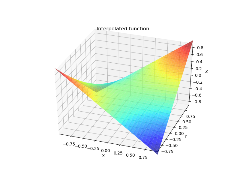
Create a b-spline from the a meshgrid of 50 points in the x-direction and y-direction between -1 and 1 of the function `z=x y`.
import numpy as np
import matplotlib.pyplot as plt
from mpl_toolkits.mplot3d.axes3d import Axes3D
from matplotlib import cm
#%% Define function over 50x50 grid
xgrid = np.linspace(-1, 1, 50)
ygrid = xgrid
x, y = np.meshgrid(xgrid, ygrid)
z = x*y
fig = plt.figure(figsize=(8, 6))
ax = fig.add_subplot(111, projection='3d')
ax.plot_surface(x,
y,
z,
rstride=2, cstride=2,
cmap=cm.jet,
alpha=0.7,
linewidth=0.25)
plt.title('Sparsely sampled function')
ax.set_xlabel('X')
ax.set_ylabel('Y')
ax.set_zlabel('Z')
#%% Interpolate function over new 70x70 grid
xgrid2 = np.linspace(-1, 1, 70)
ygrid2 = xgrid2
xnew,ynew = np.meshgrid(xgrid2, ygrid2, indexing='ij')
tck = bisplrep(x, y, z, s=0.1) # Build the spline
znew = bisplev(xnew[:,0], ynew[0,:], tck) # Evaluate the spline
fig = plt.figure(figsize=(8, 6))
ax = fig.add_subplot(111, projection='3d')
ax.plot_surface(xnew,
ynew,
znew,
rstride=2, cstride=2,
cmap=cm.jet,
alpha=0.7,
linewidth=0.25)
plt.title('Interpolated function')
ax.set_xlabel('X')
ax.set_ylabel('Y')
ax.set_zlabel('Z')
plt.show()
When creating a bspline object, there are two ways to define the bspline. The first is to define the knots and coefficients directly. Three variables are created as part of the object including:
- object_name.x
- object_name.y
- object_name.z
The x and y are the independent parameters and the z is the dependent variable that is the result of the b-spline evaluation.
import numpy as np
#knots and coeffs
m = GEKKO(remote=False)
tx = [ -1, -1, -1, -1, 1, 1, 1, 1]
ty = [ -1, -1, -1, -1, 1, 1, 1, 1]
c = [1.0, 0.33333333, -0.33333333, -1.0, 0.33333333, 0.11111111, -0.11111111,
-0.33333333, -0.33333333, -0.11111111, 0.11111111, 0.33333333, -1.0, -0.33333333,
0.33333333, 1.0]
x = m.Var(0.5,-1,1)
y = m.Var(0.5,-1,1)
z = m.Var(2)
m.bspline(x,y,z,tx,ty,c,data=False)
m.Minimize(z)
m.solve()
Three files are required including for an APMonitor implementation including:
- object_name_tx.csv (x direction knots)
- object_name_ty.csv (y direction knots)
- object_name_c.csv (b-spline coefficients)
The knots and coefficients can be generated from packages such as Python or MATLAB.
File b_tx.csv
-1
-1
-1
-1
1
1
1
1
End File
! y direction knots
File b_ty.csv
-1
-1
-1
-1
1
1
1
1
End File
! b-spline coefficients
File b_c.csv
1.0
0.33333333
-0.33333333
-1.0
0.33333333
0.11111111
-0.11111111
-0.33333333
-0.33333333
-0.11111111
0.11111111
0.33333333
-1.0
-0.33333333
0.33333333
1.0
End File
Objects
b = bspline
End Objects
Connections
x = b.x
y = b.y
z = b.z
Parameters
x = 0.5 > -1 < 1
y = -0.5 > -1 < 1
Variables
z = 2.0
Equations
minimize z
The second method is to feed in the raw data and let APMonitor or GEKKO generate the knots and coefficients.
import numpy as np
m = GEKKO(remote=False)
xgrid = np.linspace(-1, 1, 20)
ygrid = xgrid
xg,yg = np.meshgrid(xgrid,ygrid)
z_data = xg*yg
x = m.Var(0.5,-1,1)
y = m.Var(0.5,-1,1)
z = m.Var(2)
m.bspline(x,y,z,xgrid,ygrid,z_data)
m.Minimize(z)
m.solve()
Three files are required for the APMonitor implementation including:
- object_name_x.csv (x direction mesh points as 1D vector)
- object_name_y.csv (y direction mesh points as 1D vector)
- object_name_z.csv (z direction mesh grid evaluations as 2D matrix)
! x direction points
File b_x.csv
-1.000000000000000000e+00
-9.591836734693877098e-01
-9.183673469387755306e-01
-8.775510204081632404e-01
-8.367346938775510612e-01
-7.959183673469387710e-01
-7.551020408163264808e-01
-7.142857142857143016e-01
-6.734693877551021224e-01
-6.326530612244898322e-01
-5.918367346938775420e-01
-5.510204081632653628e-01
-5.102040816326530726e-01
-4.693877551020408934e-01
-4.285714285714286031e-01
-3.877551020408164240e-01
-3.469387755102041337e-01
-3.061224489795918435e-01
-2.653061224489796643e-01
-2.244897959183673741e-01
-1.836734693877551949e-01
-1.428571428571429047e-01
-1.020408163265307255e-01
-6.122448979591843532e-02
-2.040816326530614511e-02
2.040816326530614511e-02
6.122448979591821328e-02
1.020408163265305035e-01
1.428571428571427937e-01
1.836734693877550839e-01
2.244897959183671521e-01
2.653061224489794423e-01
3.061224489795917325e-01
3.469387755102040227e-01
3.877551020408163129e-01
4.285714285714283811e-01
4.693877551020406713e-01
5.102040816326529615e-01
5.510204081632652517e-01
5.918367346938773199e-01
6.326530612244896101e-01
6.734693877551019003e-01
7.142857142857141906e-01
7.551020408163264808e-01
7.959183673469385489e-01
8.367346938775508391e-01
8.775510204081631294e-01
9.183673469387754196e-01
9.591836734693877098e-01
1.000000000000000000e+00
End File
! y direction points
File b_y.csv
-1.000000000000000000e+00
-9.591836734693877098e-01
-9.183673469387755306e-01
-8.775510204081632404e-01
-8.367346938775510612e-01
-7.959183673469387710e-01
-7.551020408163264808e-01
-7.142857142857143016e-01
-6.734693877551021224e-01
-6.326530612244898322e-01
-5.918367346938775420e-01
-5.510204081632653628e-01
-5.102040816326530726e-01
-4.693877551020408934e-01
-4.285714285714286031e-01
-3.877551020408164240e-01
-3.469387755102041337e-01
-3.061224489795918435e-01
-2.653061224489796643e-01
-2.244897959183673741e-01
-1.836734693877551949e-01
-1.428571428571429047e-01
-1.020408163265307255e-01
-6.122448979591843532e-02
-2.040816326530614511e-02
2.040816326530614511e-02
6.122448979591821328e-02
1.020408163265305035e-01
1.428571428571427937e-01
1.836734693877550839e-01
2.244897959183671521e-01
2.653061224489794423e-01
3.061224489795917325e-01
3.469387755102040227e-01
3.877551020408163129e-01
4.285714285714283811e-01
4.693877551020406713e-01
5.102040816326529615e-01
5.510204081632652517e-01
5.918367346938773199e-01
6.326530612244896101e-01
6.734693877551019003e-01
7.142857142857141906e-01
7.551020408163264808e-01
7.959183673469385489e-01
8.367346938775508391e-01
8.775510204081631294e-01
9.183673469387754196e-01
9.591836734693877098e-01
1.000000000000000000e+00
End File
! evaluation of function for x and y meshgrid
File b_z.csv
! all the z data as a matrix (really long)
End File
Objects
b = bspline
End Objects
Connections
x = b.x
y = b.y
z = b.z
Parameters
x = 0.5 > -1 < 1
y = -0.5 > -1 < 1
Variables
z = 2.0
Equations
minimize z
See also C-Spline Object for 1D function approximations from data