
 Type: Object
 Data: A, B, C, D, and E matrices
 Inputs: Input (u)
 Outputs: States (x), Output (y)
 Description: LTI State Space Model
 APMonitor Usage: sys = lti
 GEKKO Usage: x,y,u = m.state_space(A,B,C,D=None)
 Other optional arguments: E=None,discrete=False,dense=False
Linear Time Invariant (LTI) state space models are a linear representation of a dynamic system in either discrete or continuous time. Putting a model into state space form is the basis for many methods in process dynamics and control analysis. Below is the continuous time form of a model in state space form.
$$E\dot x = A x + B u$$
$$y = C x + D u$$
with states `x in \mathbb{R}^n` and state derivatives `\dot x = {dx}/{dt} in \mathbb{R}^n`. The notation `in \mathbb{R}^n` means that `x` and `\dot x` are in the set of real-numbered vectors of length `n`. The other elements are the outputs `y in \mathbb{R}^p`, the inputs `u in \mathbb{R}^m`, the state transition matrix `A`, the input matrix `B`, and the output matrix `C`. The remaining matrix `D` is typically zeros because the inputs do not typically affect the outputs directly. The dimensions of each matrix are shown below with `m` inputs, `n` states, and `p` outputs.
$$A \in \mathbb{R}^{n \, \mathrm{x} \, n}$$ $$B \in \mathbb{R}^{n \, \mathrm{x} \, m}$$ $$C \in \mathbb{R}^{p \, \mathrm{x} \, n}$$ $$D \in \mathbb{R}^{p \, \mathrm{x} \, m}$$ $$E \in \mathbb{R}^{n \, \mathrm{x} \, n}$$
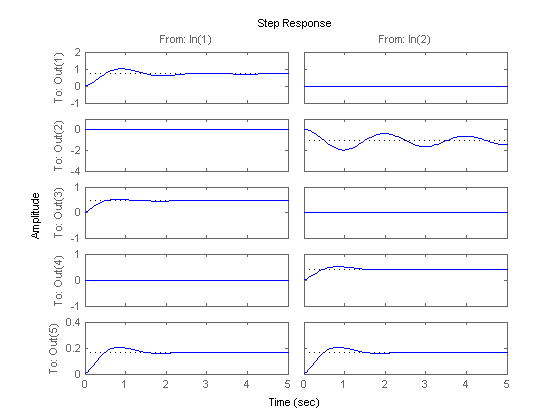
Model Predictive Control, or MPC, is an advanced method of process control that has been in use in the process industries such as chemical plants and oil refineries since the 1980s. Model predictive controllers rely on dynamic models of the process, most often linear empirical models obtained by system identification.
These models are typically in the finite impulse response form or linear state space form. Either model form can be converted to an APMonitor for a linear MPC upgrade. Once in APMonitor form, nonlinear elements can be added to avoid multiple model switching, gain scheduling, or other ad hoc measures commonly employed because of linear MPC restrictions.
Example Model in APMonitor
 ! new linear time-invariant object
 Model control
   Objects
     mpc = lti
   End Objects
 End Model

 ! Model information
 ! continuous form
 ! dx/dt = A * x + B * u
 !     y = C * x + D * u
 !
 ! dimensions
 ! (nx1) = (nxn)*(nx1) + (nxm)*(mx1)
 ! (px1) = (pxn)*(nx1) + (pxm)*(mx1)
 !
 ! discrete form
 ! x[k+1] = A * x[k] + B * u[k]
 !   y[k] = C * x[k] + D * u[k]
 File mpc.txt
   sparse, continuous  ! dense/sparse, continuous/discrete
   2      ! m=number of inputs
   3      ! n=number of states
   3      ! p=number of outputs
 End File

 ! A matrix (row, column, value)
 File mpc.a.txt
   1  1  0.9
   2  2  0.1
   3  3  0.5
 End File

 ! B matrix (row, column, value)
 File mpc.b.txt
   1  1  1.0
   2  2  1.0
   3  1  0.5
   3  2  0.5
 End File

 ! C matrix (row, column, value)
 File mpc.c.txt
   1  1  0.5
   2  2  1.0
   3  3  2.0
 End File

 ! D matrix (row, column, value)
 File mpc.d.txt
   1  1  0.2
 End File
Example Model Predictive Control in GEKKO
from gekko import GEKKO
A = np.array([[-.003, 0.039, 0, -0.322],
[-0.065, -0.319, 7.74, 0],
[0.020, -0.101, -0.429, 0],
[0, 0, 1, 0]])
B = np.array([[0.01, 1, 2],
[-0.18, -0.04, 2],
[-1.16, 0.598, 2],
[0, 0, 2]]
)
C = np.array([[1, 0, 0, 0],
[0, -1, 0, 7.74]])
#%% Build GEKKO State Space model
m = GEKKO()
x,y,u = m.state_space(A,B,C,D=None)
# customize names
# MVs
mv0 = u[0]
mv1 = u[1]
# Feedforward
ff0 = u[2]
# CVs
cv0 = y[0]
cv1 = y[1]
m.time = [0, 0.1, 0.2, 0.4, 1, 1.5, 2, 3, 4]
m.options.imode = 6
m.options.nodes = 3
u[0].lower = -5
u[0].upper = 5
u[0].dcost = 1
u[0].status = 1
u[1].lower = -5
u[1].upper = 5
u[1].dcost = 1
u[1].status = 1
## CV tuning
# tau = first order time constant for trajectories
y[0].tau = 5
y[1].tau = 8
# tr_init = 0 (dead-band)
# = 1 (first order trajectory)
# = 2 (first order traj, re-center with each cycle)
y[0].tr_init = 0
y[1].tr_init = 0
# targets (dead-band needs upper and lower values)
# SPHI = upper set point
# SPLO = lower set point
y[0].sphi= -8.5
y[0].splo= -9.5
y[1].sphi= 5.4
y[1].splo= 4.6
y[0].status = 1
y[1].status = 1
# feedforward
u[2].status = 0
u[2].value = np.zeros(np.size(m.time))
u[2].value[3:] = 2.5
m.solve() # (GUI=True)
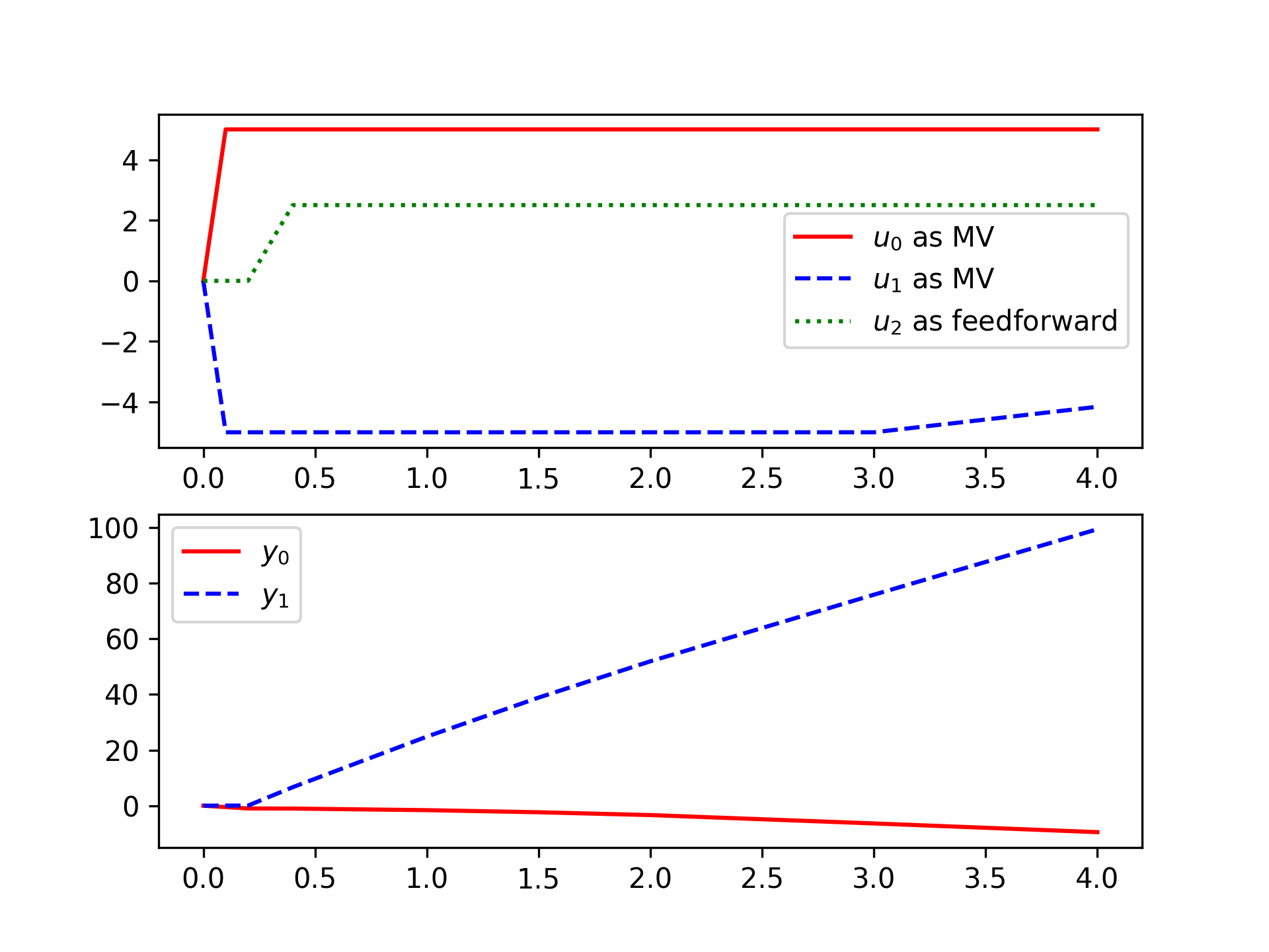
# also create a Python plot
import matplotlib.pyplot as plt
plt.subplot(2,1,1)
plt.plot(m.time,mv0.value,'r-',label=r'$u_0$ as MV')
plt.plot(m.time,mv1.value,'b--',label=r'$u_1$ as MV')
plt.plot(m.time,ff0.value,'g:',label=r'$u_2$ as feedforward')
plt.legend()
plt.subplot(2,1,2)
plt.plot(m.time,cv0.value,'r-',label=r'$y_0$')
plt.plot(m.time,cv1.value,'b--',label=r'$y_1$')
plt.legend()
plt.show()
Also see: