APMonitor

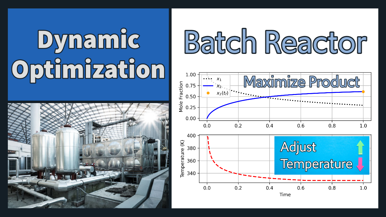
Batch reactors are pre-loaded with reactants and undergo processing steps to produce a final product in a finite time. Batch reactors are typical for smaller or high-value production processes where the reactor is loaded, processed, and product removed from the reactor to prepare for the next batch. Batch reactors are common in chemical and pharmaceutical manufacture, biofuel production, food and beverage industries, and agricultural production.

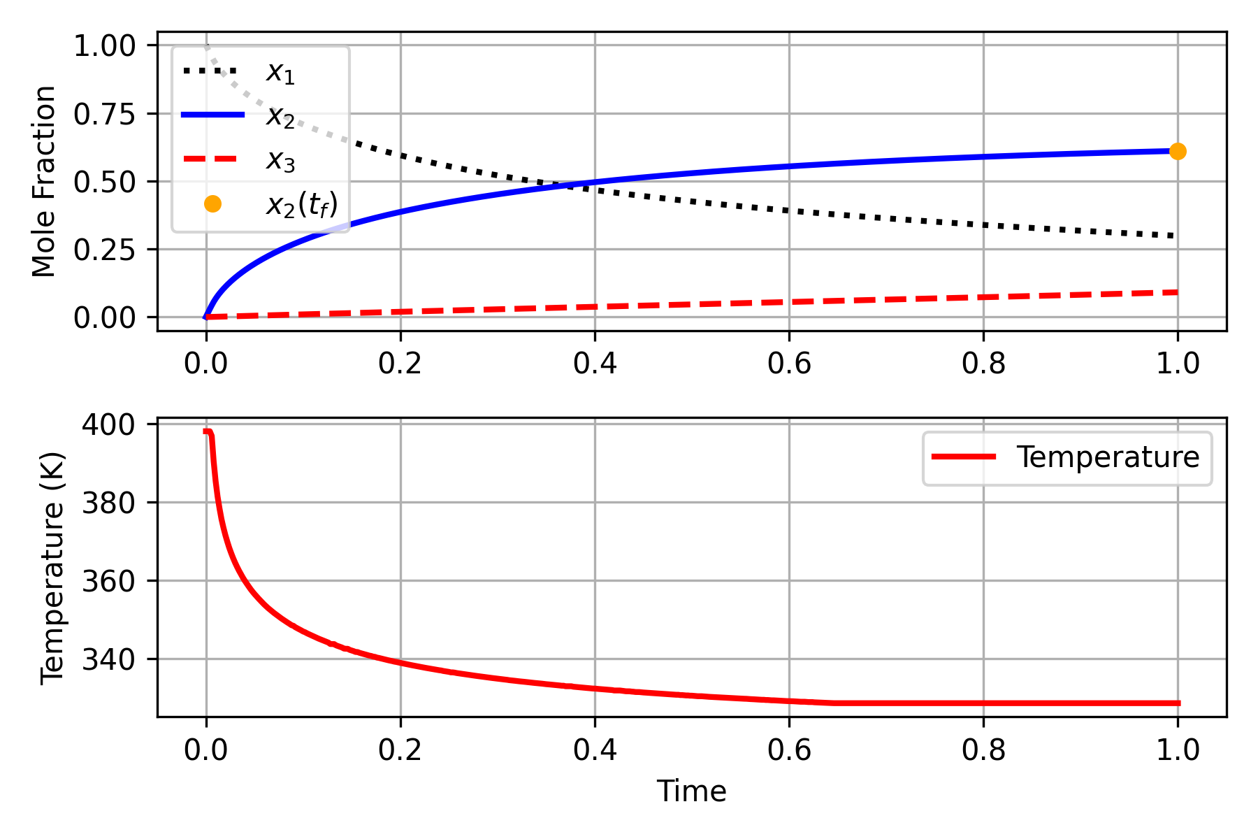
This batch reactor problem describes the reaction of reactant A that produces intermediate B as the desired product. A second reaction converts B into an undesirable product C. The batch reactor temperature is continuously controlled with a cooling jacket throughout the time window. A mathematical statement of the optimal control problem is given by

$$\begin{array}{llcl}\max_{x,u} & x_2(t_f) \\ \mbox{s.t.} & \frac{dx_1}{dt} & = & -k_1 x_1^2\\ & \frac{dx_2}{dt} & = & k_1 x_1^2 - k_2 x_2\\ & \frac{dx_3}{dt} & = & k_2 x_2 \\ & k_1 & = & 4000 \; e^{-2500/T(t)}\\ & k_2 & = & 620000 \; e^{-5000/T(t)}\\ & x(0) &=& (1, 0)^T\\ & T(t) &\in& [298, 398]\end{array}$$

where `x_1(t)` is the concentration of A, `x_2(t)` is the concentration of B, and `x_3(t)` is the concentration of C at time-point t. The control function T(t) is the temperature. The starting time is 0 and end time is 1.

The optimal objective value of the problem is x2(tf) = 0.6108.

The Gekko Optimization Suite is a machine learning and optimization package in Python for mixed-integer and differential algebraic equations.

📄 Gekko Publication and References

The GEKKO package is available in Python with pip install gekko. There are additional example problems for equation solving, optimization, regression, dynamic simulation, model predictive control, and machine learning.