Biomechanic Regression


Biomechanics is the study of the mechanical principles that govern human movement, such as the forces and motions involved in walking, running, jumping, and other physical activities. It is an interdisciplinary field that combines principles from physics, engineering, and anatomy to understand how the body moves and functions. Biomechanics is used in many areas, including sports science, rehabilitation, ergonomics, and robotics.
An application of biomechanics is predicting the peak force of a runner's stride. Features such as angles, hip flexion, leg lift, and speed determine the maximum force that a runner's body generates during a stride. This information is useful for coaches and athletes who want to optimize training and performance by identifying areas of weakness and improving biomechanics. By analyzing the biomechanics of a runner's stride, a coach can identify areas of inefficiency or improper technique that may increase the risk of injury. With this information, the coach can work with the athlete to modify their running technique or develop strength training exercises to improve weak areas.
Objective: Predict peak force (lpeakforce) of a runner's stride using the 10 features in the data file that are collected from several runners at various speeds. See the Running Mechanics website for more description of the data.

Features (Inputs)
- lgt = left leg ground contact time
- sr = stride rate
- sl = stride length
- lkneeswing – left knee angle during the swing phase (maximum flexion during time off ground)
- lhipflex – left hip maximum flexion
- lhipext – left hip maximum hyperextension
- lcmvert – vertical oscillation of the center of mass when coming off the left foot
- lkneesep – horizontal forward displacement between knees when leaving the ground on the left foot
- lcmtoe – horizontal forward displacement between center of mass and left toe as it touches the ground
Target (Output)
- lpeakforce - left leg peak force
The process for data regression includes importing and cleaning data, scaling the data, splitting it into train and test sets, selecting important features, and evaluating the accuracy of the model using a suitable metric. See Machine Learning for Engineers for an overview of how to process data for classification and regression.
Data and Package Import
Import the data with pandas as a DataFrame. Use pip install lazypredict to install a package that evaluates all regressors in scikit-learn.
import pandas as pd
import matplotlib.pyplot as plt
from sklearn.preprocessing import StandardScaler
from sklearn.feature_selection import SelectKBest
from sklearn.feature_selection import f_regression
from lazypredict.Supervised import LazyRegressor
url = 'http://apmonitor.com/dde/uploads/Main/biomechanics.txt'
data = pd.read_csv(url)
data.head()
Data Cleansing
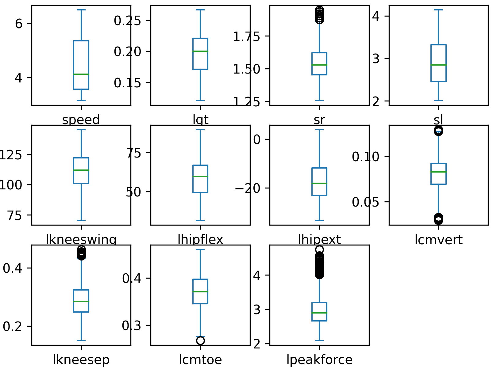
Data cleansing identifies and corrects errors in the data, such as missing values, duplicates, and outliers. This step is crucial for ensuring that the data is accurate and reliable.
data.dropna(inplace=True)
# lgt > 0
data = data[data['lgt']>0]
# 0 < left knee swing < 150
data = data[(data['lkneeswing']>0)&(data['lkneeswing']<150)]
# create boxplot to identify any other outliers
data.plot(kind='box',subplots=True,layout=(3,4))
plt.savefig('boxplot.png',dpi=300)
Scale and Shuffle Data
Scaling the data ensures that all the features are in the same range and improves certain regressors such as Neural Networks. This step is important for preventing bias in the model and improving accuracy. Shuffling ensures that data order is randomized.
data = data.sample(frac=1).reset_index(drop=True)
# standard scaler: mean=0, standard deviation=1
s = StandardScaler()
s_data = s.fit_transform(data)
Split Data into Train and Test Sets
Data is split into two sets: the training set and the testing set. The training set is used to train the model, while the testing set is used to evaluate accuracy.
X = s_data[:,0:-1]; y = s_data[:,-1]
# 80% for training, 20% for testing
split = int(X.shape[0] * 0.8)
X_train, y_train = X[:split], y[:split]
X_test, y_test = X[split:], y[split:]
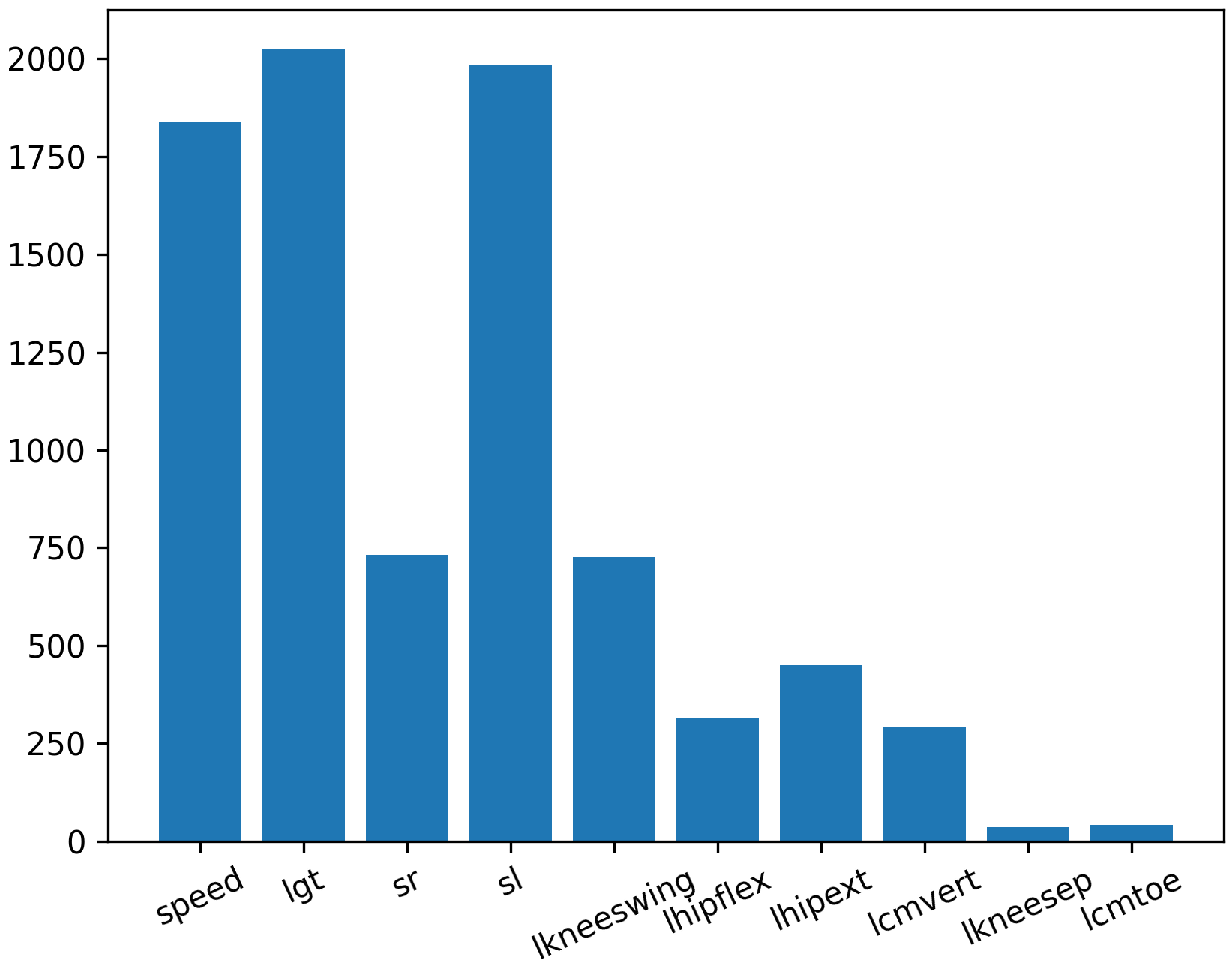
Feature Ranking
Feature ranking selects the most important features that are highly correlated to the predicted variable. This step helps to reduce the complexity of the model and improve accuracy by keeping only the most important features.
fs = SelectKBest(score_func=f_regression, k='all')
# learn relationship from training data
fs.fit(X_train, y_train)
# scores for the features
cn = data.columns
for i in range(len(fs.scores_)):
print('Feature %s: %f' % (cn[i], fs.scores_[i]))
plt.figure()
plt.bar([i for i in range(len(fs.scores_))], fs.scores_)
ax = plt.gca()
idx = np.arange(0,X.shape[1])
ax.set_xticks(idx)
ax.set_xticklabels(cn[0:-1], rotation=25)
plt.savefig('best_features.png',dpi=300)
Quantify Accuracy
Use all regressors in the scikit-learn package. The accuracy of the model is evaluated using a suitable metric, such as the mean squared error (MSE) or R-squared. The scikit-learn package provides several regressors that can be used for data regression, including linear regression, decision trees, and support vector regressors.
reg = LazyRegressor(verbose=0, ignore_warnings=False, custom_metric=None)
models, predictions = reg.fit(X_train, X_test, y_train, y_test)
models.to_csv('reg_train.csv')
print(models)
| Model | Adjusted R-Squared | R-Squared | RMSE | Time Taken |
|---|---|---|---|---|
| ExtraTreesRegressor | 0.94 | 0.94 | 0.24 | 0.57 |
| KNeighborsRegressor | 0.92 | 0.93 | 0.27 | 0.01 |
| RandomForestRegressor | 0.92 | 0.93 | 0.27 | 1.65 |
| HistGradientBoostingRegressor | 0.92 | 0.92 | 0.28 | 0.59 |
| LGBMRegressor | 0.92 | 0.92 | 0.29 | 0.08 |
| BaggingRegressor | 0.91 | 0.92 | 0.29 | 0.17 |
| XGBRegressor | 0.91 | 0.91 | 0.3 | 0.14 |
| MLPRegressor | 0.9 | 0.9 | 0.31 | 1.46 |
| SVR | 0.89 | 0.89 | 0.33 | 0.19 |
| NuSVR | 0.89 | 0.89 | 0.33 | 0.23 |
| GradientBoostingRegressor | 0.86 | 0.86 | 0.37 | 0.62 |
| GaussianProcessRegressor | 0.86 | 0.86 | 0.37 | 0.29 |
| ExtraTreeRegressor | 0.84 | 0.84 | 0.39 | 0.01 |
| DecisionTreeRegressor | 0.82 | 0.82 | 0.42 | 0.02 |
| AdaBoostRegressor | 0.74 | 0.74 | 0.51 | 0.17 |
| BayesianRidge | 0.64 | 0.64 | 0.59 | 0.01 |
| ElasticNetCV | 0.64 | 0.64 | 0.59 | 0.07 |
| LassoCV | 0.64 | 0.64 | 0.59 | 0.06 |
| RidgeCV | 0.64 | 0.64 | 0.59 | 0.01 |
| Ridge | 0.64 | 0.64 | 0.59 | 0.01 |
| Lars | 0.64 | 0.64 | 0.59 | 0.01 |
| TransformedTargetRegressor | 0.64 | 0.64 | 0.59 | 0.01 |
| LarsCV | 0.64 | 0.64 | 0.59 | 0.02 |
| LassoLarsCV | 0.64 | 0.64 | 0.59 | 0.02 |
| LinearRegression | 0.64 | 0.64 | 0.59 | 0.01 |
| LassoLarsIC | 0.64 | 0.64 | 0.59 | 0.01 |
| KernelRidge | 0.64 | 0.64 | 0.59 | 0.14 |
| SGDRegressor | 0.63 | 0.64 | 0.6 | 0.01 |
| HuberRegressor | 0.6 | 0.61 | 0.62 | 0.03 |
| LinearSVR | 0.6 | 0.61 | 0.62 | 0.02 |
| OrthogonalMatchingPursuitCV | 0.6 | 0.61 | 0.62 | 0.01 |
| TweedieRegressor | 0.55 | 0.56 | 0.66 | 0.01 |
| OrthogonalMatchingPursuit | 0.5 | 0.51 | 0.7 | 0.01 |
| RANSACRegressor | 0.36 | 0.37 | 0.79 | 0.1 |
| PassiveAggressiveRegressor | 0.27 | 0.28 | 0.84 | 0.01 |
| ElasticNet | 0.21 | 0.22 | 0.88 | 0.01 |
| DummyRegressor | -0.02 | 0 | 1 | 0.01 |
| LassoLars | -0.02 | 0 | 1 | 0.01 |
| Lasso | -0.02 | 0 | 1 | 0.01 |
| QuantileRegressor | -0.03 | -0.01 | 1 | 167.62 |
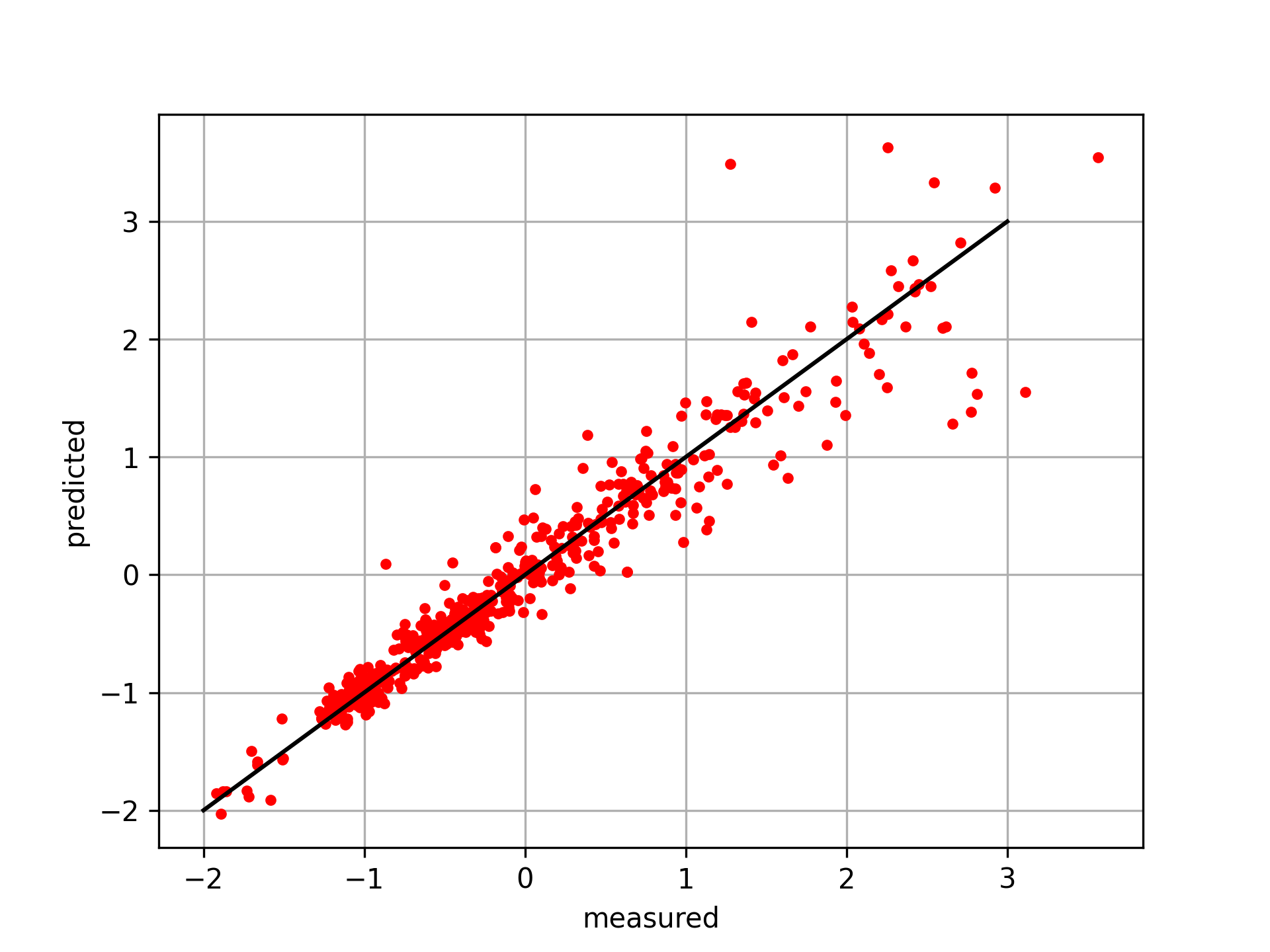
Select Regressor and Evaluate Test Data
from sklearn.neighbors import KNeighborsRegressor
knn = KNeighborsRegressor(n_neighbors=5)
knn.fit(X_train,y_train)
y_pred = knn.predict(X_test)
# plot results
plt.figure()
plt.plot(y_test,y_pred,'r.')
plt.plot([-2,3],[-2,3],'k-')
plt.xlabel('measured'); plt.ylabel('predicted')
plt.grid(); plt.savefig('predict.png',dpi=300)
plt.show()
import pandas as pd
import matplotlib.pyplot as plt
from sklearn.preprocessing import StandardScaler
from sklearn.feature_selection import SelectKBest
from sklearn.feature_selection import f_regression
from lazypredict.Supervised import LazyRegressor
url = 'http://apmonitor.com/dde/uploads/Main/biomechanics.txt'
data = pd.read_csv(url)
data.head()
# drop bad data rows
data.dropna(inplace=True)
# lgt > 0
data = data[data['lgt']>0]
# 0 < left knee swing < 150
data = data[(data['lkneeswing']>0)&(data['lkneeswing']<150)]
# create boxplot to identify any other outliers
data.plot(kind='box',subplots=True,layout=(3,4))
plt.savefig('boxplot.png',dpi=300)
# shuffle rows
data = data.sample(frac=1).reset_index(drop=True)
# standard scaler: mean=0, standard deviation=1
s = StandardScaler()
s_data = s.fit_transform(data)
# features and target
X = s_data[:,0:-1]; y = s_data[:,-1]
# 80% for training, 20% for testing
split = int(X.shape[0] * 0.8)
X_train, y_train = X[:split], y[:split]
X_test, y_test = X[split:], y[split:]
# best features
fs = SelectKBest(score_func=f_regression, k='all')
# learn relationship from training data
fs.fit(X_train, y_train)
# scores for the features
cn = data.columns
for i in range(len(fs.scores_)):
print('Feature %s: %f' % (cn[i], fs.scores_[i]))
plt.figure()
plt.bar([i for i in range(len(fs.scores_))], fs.scores_)
ax = plt.gca()
idx = np.arange(0,X.shape[1])
ax.set_xticks(idx)
ax.set_xticklabels(cn[0:-1], rotation=25)
plt.savefig('best_features.png',dpi=300)
# fit all regressors
reg = LazyRegressor(verbose=0, ignore_warnings=False, custom_metric=None)
models, predictions = reg.fit(X_train, X_test, y_train, y_test)
models.to_csv('reg_train.csv')
print(models)
# fit and test with kNN
from sklearn.neighbors import KNeighborsRegressor
knn = KNeighborsRegressor(n_neighbors=5)
knn.fit(X_train,y_train)
y_pred = knn.predict(X_test)
# plot results
plt.figure()
plt.plot(y_test,y_pred,'r.')
plt.plot([-2,3],[-2,3],'k-')
plt.xlabel('measured'); plt.ylabel('predicted')
plt.grid(); plt.savefig('predict.png',dpi=300)
plt.show()
Challenge Problem: Predict Both Left and Right Peak Force
The biomechanics regression example predicted only left peak force (lpeakforce) from stride / joint / COM features. In this challenge, extend the workflow to predict both:
- lpeakforce: left leg peak force
- rpeakforce: right leg peak force
Build two separate regression models (one per target) and compare many scikit-learn regressors in ranked order to identify the best-performing approach for each target.
Tasks
- Load and clean the dataset
- Remove invalid or impossible rows (e.g., missing values, negative contact time, implausible angles).
- Ensure the final dataset contains both targets: lpeakforce and rpeakforce.
- Prepare the inputs
- Use the available biomechanical features as inputs (e.g., ground contact time, stride rate, stride length, joint angles, COM oscillation / displacement measures).
- Do not include the target you are predicting as an input feature.
- Train / test split
- Split the dataset into training and test sets (e.g., 80/20).
- Standardize features (and optionally targets) to support regressors that benefit from scaling.
- Benchmark regressors (ranked order)
- Use LazyRegressor (or an equivalent loop) to train and score a wide set of regressors.
- Rank models by a primary metric (recommend: R² or RMSE) on the test set.
- Produce a table of the top models for lpeakforce prediction and rpeakforce prediction
- Find the best features for each target
- Compute feature relevance separately for each target (e.g., SelectKBest(f_regression)).
- Report the top features (by score) for lpeakforce and rpeakforce
- Discuss whether the best features are the same or different between left and right.
Deliverables
- Model leaderboard (two tables)
- Ranked regressors for predicting lpeakforce
- Ranked regressors for predicting rpeakforce
- Include at least: Adjusted R² (if available), R², RMSE, time taken.
- Feature ranking (two lists + plots)
- Top features for lpeakforce (with scores)
- Top features for rpeakforce (with scores)
- Best model selection
- Identify the top regressor for each target.
- Briefly justify why it wins (accuracy vs complexity vs runtime).
- Optional: show predicted vs measured scatter plots for the best model(s).
Evaluation Criteria
- Correct data preprocessing (cleaning + split + scaling)
- Proper model comparison (same split, same metric, consistent pipeline)
- Clear ranked results for both targets
- Separate feature selection for left and right targets
- Quality of interpretation (what features matter most and why)
Hint
Many biomechanics relationships are nonlinear. Ensemble tree methods (e.g., ExtraTrees / RandomForest) and kernel methods (SVR) often perform well. Compare accuracy and runtime, and verify that you are not leaking targets into inputs.
Solution Overview

This solution follows a standard supervised-learning workflow to predict left and right peak force from running kinematics:
- Load and clean the data (remove non-numeric identifiers, handle missing values).
- Create two modeling problems:
- Inputs X = biomechanical features
- Targets `y_L` = lpeakforce, `y_R` = rpeakforce
- Train/test split (80/20) and standardize inputs (and optionally targets for model screening).
- Evaluate many regressors in ranked order for each target using LazyPredict.
- Rank features separately for each target using SelectKBest(f_regression).
- Report the best regressor and the top features for each target.
Key Outputs to Report
- Top-ranked regressors for lpeakforce and rpeakforce (R² / RMSE).
- Best model choice for each.
- Top features for each target (they may differ because the runner can load left/right asymmetrically).
Source Code
import numpy as np
import matplotlib.pyplot as plt
import seaborn as sns
from sklearn.model_selection import train_test_split
from sklearn.linear_model import LinearRegression
from sklearn.ensemble import RandomForestRegressor
from sklearn.metrics import mean_absolute_error, mean_squared_error, r2_score
from lazypredict.Supervised import LazyRegressor, REGRESSORS
from sklearn.preprocessing import StandardScaler
from sklearn.feature_selection import SelectKBest, f_regression
# Set plot style
sns.set_theme(style="whitegrid")
def load_and_clean_data(filepath):
"""Loads the dataset and performs initial cleaning."""
print(f"Loading data from {filepath}...")
df = pd.read_csv(filepath)
# Drop non-numeric identifier columns that are unlikely to be predictive
drop_cols = ['ID', 'username', 'fname', 'lname', 'email']
df_cleaned = df.drop(columns=[c for c in drop_cols if c in df.columns])
# Check for missing values
print("\nMissing values per column:")
print(df_cleaned.isnull().sum())
# Fill missing values with median for numeric columns (simple imputation)
# Only if there are any
if df_cleaned.isnull().values.any():
print("\nImputing missing values with median...")
for col in df_cleaned.select_dtypes(include=np.number).columns:
df_cleaned[col] = df_cleaned[col].fillna(df_cleaned[col].median())
return df_cleaned
def visualize_data(df, targets=['lpeakforce', 'rpeakforce']):
"""Generates visualizations for the data."""
print("\nGenerating visualizations...")
# 1. Correlation Matrix
plt.figure(figsize=(12, 10))
# Select only numeric columns for correlation
numeric_df = df.select_dtypes(include=np.number)
corr = numeric_df.corr()
sns.heatmap(corr, annot=False, cmap='coolwarm', fmt=".2f")
plt.title('Correlation Matrix')
plt.tight_layout()
plt.savefig('correlation_matrix.png')
print("Saved correlation_matrix.png")
# 2. Distribution of Target Variables
for target in targets:
if target in df.columns:
plt.figure(figsize=(8, 6))
sns.histplot(df[target], kde=True, bins=30)
plt.title(f'Distribution of {target}')
plt.tight_layout()
plt.savefig(f'distribution_{target}.png')
print(f"Saved distribution_{target}.png")
# 3. Scatter plots against highest correlated feature (excluding targets)
for target in targets:
if target in df.columns:
# Drop all target columns from the candidates (and itself obviously)
# We want the highest correlation with a FEATURE, not another target
candidates = corr[target].drop(labels=[t for t in targets if t in corr.index], errors='ignore')
if not candidates.empty:
best_feature = candidates.abs().idxmax()
plt.figure(figsize=(8, 6))
sns.scatterplot(data=df, x=best_feature, y=target)
plt.title(f'{target} vs {best_feature}')
plt.tight_layout()
plt.savefig(f'scatter_{target}_vs_{best_feature}.png')
print(f"Saved scatter_{target}_vs_{best_feature}.png")
def train_and_evaluate(df, target_col):
"""Trains regression models and evaluates them."""
print(f"\n--- Analysis for Target: {target_col} ---")
# Separate features and target
X = df.drop(columns=['lpeakforce', 'rpeakforce']) # Drop both targets from features to avoid leakage
# We might want to keep other 'left' variables for 'left' target?
# Usually in these biomechanics datasets, knowing the counterpart might be 'cheating'
# or it might be a requirement. For now, I'll drop the OTHER target from features,
# but keep all other columns.
# Ensure all X are numeric
X = X.select_dtypes(include=np.number)
y = df[target_col]
# Split data
X_train, X_test, y_train, y_test = train_test_split(X, y, test_size=0.2, random_state=42)
# Lazy Predict Integration
print("\n--- Running Lazy Predict ---")
reg_select = []
exclude = ['LGBMRegressor', 'GammaRegressor', 'PoissonRegressor']
for x in REGRESSORS:
if not any(x[0] == ex for ex in exclude):
reg_select.append(x[1])
# LazyRegressor doesn't handle scaling automatically in the way requested?
# User example scaled data manually. Let's follow that pattern or check if necessary.
# User code:
# s0 = StandardScaler(); s1 = StandardScaler()
# Xs = s0.fit_transform(X); ys = s1.fit_transform(y)
# Xs_train, Xs_test, ys_train, ys_test = train_test_split(Xs, ys ...)
# Since I already split X_train, X_test, y_train, y_test (unscaled), I should scale them for LazyPredict as per user request
# Note: X_train and X_test are DataFrames, y_train and y_test are Series.
scaler_X = StandardScaler()
scaler_y = StandardScaler()
X_train_scaled = scaler_X.fit_transform(X_train)
X_test_scaled = scaler_X.transform(X_test)
# Reshape y for scaling
y_train_scaled = scaler_y.fit_transform(y_train.values.reshape(-1, 1))
y_test_scaled = scaler_y.transform(y_test.values.reshape(-1, 1))
# Initialize LazyRegressor
reg = LazyRegressor(verbose=0, ignore_warnings=False, custom_metric=None, regressors=reg_select)
# Fit
# LazyRegressor returns models and predictions
# Note: y_train, y_test in reg.fit are expected to be 1D usually, but if we scale them they become 2D arrays.
# LazyRegressor handles this? Let's check user snippet.
# User snippet: ys = s1.fit_transform(y) (ys is 2D) -> train_test_split -> ys_train (2D).
# so passing 2D array seems fine for LazyRegressor.
models_df, predictions_df = reg.fit(X_train_scaled, X_test_scaled, y_train_scaled, y_test_scaled)
print("\nLazy Predict Results (Top 5):")
print(models_df.head())
# Save results
results_filename = f'results_{target_col}.csv'
models_df.to_csv(results_filename)
print(f"Saved ranked regressors to {results_filename}")
print(f"\n--- Specific Model Evaluation (Unscaled Original) ---")
models = {
"Linear Regression": LinearRegression(),
"Random Forest": RandomForestRegressor(n_estimators=100, random_state=42)
}
results = {}
for name, model in models.items():
model.fit(X_train, y_train)
y_pred = model.predict(X_test)
mae = mean_absolute_error(y_test, y_pred)
rmse = np.sqrt(mean_squared_error(y_test, y_pred))
r2 = r2_score(y_test, y_pred)
results[name] = {'MAE': mae, 'RMSE': rmse, 'R2': r2}
print(f"\nModel: {name}")
print(f" MAE: {mae:.4f}")
print(f" RMSE: {rmse:.4f}")
print(f" R2 Score: {r2:.4f}")
# Plot Actual vs Predicted
plt.figure(figsize=(6, 6))
plt.scatter(y_test, y_pred, alpha=0.5)
plt.plot([y_test.min(), y_test.max()], [y_test.min(), y_test.max()], 'r--')
plt.xlabel('Actual')
plt.ylabel('Predicted')
plt.title(f'{name}: Actual vs Predicted ({target_col})')
plt.tight_layout()
plt.savefig(f'pred_vs_actual_{target_col}_{name.replace(" ", "_")}.png')
return results
def analyze_feature_importance(df, target_col):
"""Ranks features using SelectKBest and plots importance."""
print(f"\n--- Feature Importance Analysis for Target: {target_col} ---")
# Prepare data
X = df.drop(columns=['lpeakforce', 'rpeakforce'])
X = X.select_dtypes(include=np.number)
y = df[target_col]
# SelectKBest with f_regression
# We use k='all' to get scores for all features, then rank them
selector = SelectKBest(score_func=f_regression, k='all')
selector.fit(X, y)
# Get scores and create DataFrame
scores = selector.scores_
features = X.columns
feature_scores = pd.DataFrame({'Feature': features, 'Score': scores})
# Sort by score descending
feature_scores = feature_scores.sort_values(by='Score', ascending=False)
# Plotting Top 20 Features
plt.figure(figsize=(12, 8))
sns.barplot(x='Score', y='Feature', data=feature_scores.head(20), palette='viridis')
plt.title(f'Top 20 Features Importance for {target_col} (SelectKBest f_regression)')
plt.xlabel('F-Score')
plt.ylabel('Feature')
plt.tight_layout()
plt.savefig(f'feature_importance_{target_col}.png')
print(f"Saved feature_importance_{target_col}.png")
print("\nTop 10 Features:")
print(feature_scores.head(10))
def main():
filepath = 'biomechanics2.csv'
try:
df = load_and_clean_data(filepath)
except FileNotFoundError:
print(f"Error: {filepath} not found.")
return
visualize_data(df)
if 'lpeakforce' in df.columns:
analyze_feature_importance(df, 'lpeakforce')
train_and_evaluate(df, 'lpeakforce')
if 'rpeakforce' in df.columns:
analyze_feature_importance(df, 'rpeakforce')
train_and_evaluate(df, 'rpeakforce')
print("\nAnalysis complete.")
if __name__ == "__main__":
main()
Other Biomechanic Applications
In addition to improving performance and reducing injury risk, biomechanics can also be used to design assistive devices such as prosthetics and orthotics. By understanding the mechanical principles of human movement, engineers can design devices that mimic natural movements and provide support to individuals with physical disabilities.
Acknowledgement
Thanks to Iain Hunter of BYU Biomechanics in Exercise Science for providing the datasets.
References
- Jeong H., Park S., Estimation of the ground reaction forces from a single video camera based on the spring-like center of mass dynamics of human walking, Journal of Biomechanics, 2020 Dec Vol 2, 113, 110074. Article
- Colyer S, Needham L, Evans M, Wade L, Cosker D, Cazzola D, McGuigan P, Bilzon J. Estimation of Ground Reaction Forces from Markerless Kinematics and Comparison Against Measured Force Plate Data, ISBS Proceedings Archive, 2023, 41(1):23. Article