MPC for Copper Leaching
Copper is commonly refined from sulfide ores by acid leaching, where sulfuric acid (H2SO4) dissolves copper-bearing minerals to produce a pregnant leach solution (PLS) for downstream extraction. Copper leaching is one of the early steps in the overall copper refining chain, bridging the transition from raw ore to purified metal. After mining and crushing, copper-bearing ores (often sulfides or oxides) are subjected to leaching, where sulfuric acid dissolves the copper minerals into a pregnant leach solution (PLS). This liquid phase, enriched with dissolved copper, then passes to solvent extraction (SX), where copper is selectively transferred into an organic phase, and subsequently to electrowinning (EW), where pure copper metal is plated onto cathodes. By controlling acid concentration during leaching, operators directly influence both the efficiency of copper recovery from the ore and the stability of downstream SX–EW processes. In this way, acid regulation in leaching plays a critical role in maximizing overall recovery, minimizing chemical waste, and ensuring high-purity cathode copper production.
For copper leaching, tight regulation of acid concentration is essential. Too little acid slows leaching and leaves copper in the solids and too much acid wastes reagent, increases corrosion, and can overload neutralization steps. Ore grade and mineralogy vary over time, changing acid consumption. Because tanks are connected in series, adding more or less acid upstream propagates downstream after a residence-time delay, so a coordinated, predictive strategy (MPC) is preferred over independent PI loops.
Process & Control Objective
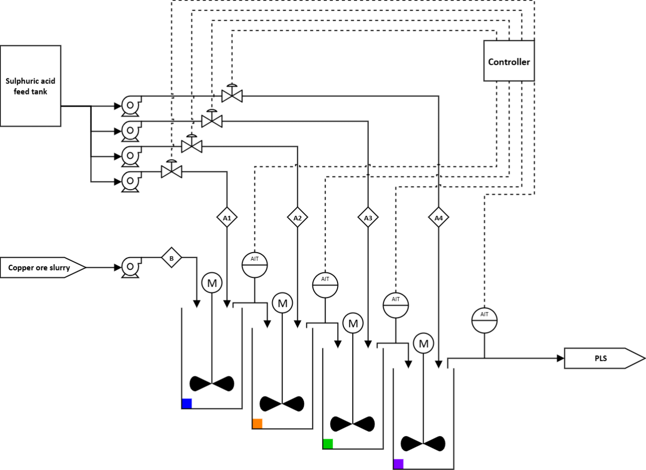
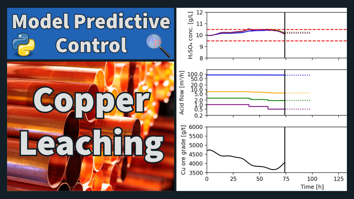
A 4-tank agitated leach train receives a copper-ore slurry feed. Each tank can receive a separate acid addition from a common H2SO4 feed system. The controller manipulates the four acid flows to keep the acid concentration for each tank within a tight deadband around a target, despite disturbances in ore copper grade (acid demand). Colors in the plots correspond to colored markers on the tanks in the P&ID.
Ore content changes acid demand
Higher copper grade (or more acid-consuming gangue) increases instantaneous acid consumption as leaching reactions proceed, effectively behaving like a sink term in the acid balance. When a higher-grade ore bump enters tank 1, locally measured acid drops. Compensating by increasing upstream acid raises the outflow acid concentration, which then increases the inflow concentration to tank 2, and so on—coupling the tanks through convection and residence-time dynamics. This cascade plus the reaction sink motivates a predictive, multi-input multi-output (MIMO) controller.
Dynamic Model (Species Balances)
For tank i with volume V and total volumetric flow Qi (including slurry and all upstream acid additions), Ci is the liquid acid concentration [g/L] and `C_{A,feed}` the acid concentration of the make-up stream. The acid addition to tank i is `F_{A,i}` [m3/h]. The leachable copper concentration is `C_i` [g/L]. A continuous stirred-tank mass balance for each tank is:
$$V\frac{dC_i}{dt}=Q_{i-1}C_{i-1} +F_{A,i} C_{A,feed} -{Q_i C_i} +r_i V$$
with `Q_0 C_0` as the slurry inflow acid term for i=1. The reaction rate that consumes acid is modeled first-order in leachable copper:
$$r_i = -k C_i \nu_A$$
where `\nu_A\approx 1.544` converts the stoichiometric acid consumption per unit copper reacted. Similar CSTR balances describe solids and leachable-copper transport and reaction:
$$V\frac{dS_i}{dt}=Q_{i-1}S_{i-1}-Q_i S_i,\qquad V\frac{dC_i}{dt}=Q_{i-1}C_{i-1}-Q_i C_i - k C_i V$$
These are the plant ODEs used for simulation and for steady-state target calculation in the Python code.
MPC Control-Oriented Simplification)
For fast optimization within the MPC, an approximate acid dynamics for each tank is a superposition of first-order responses from the acid flows that affect it (upper-triangular because upstream flows influence downstream tanks):
$$\tau_{j,i} \frac{d\tilde C_i}{dt} = -\tilde C_i + K_{j,i}\tilde F_{A,j}\qquad j\le i$$
where `\tilde C_i = C_i - \barC_i` and `\tilde F_{A,j}=F_{A,j}-\bar F_{A,j}` are deviations from steady state. Gains `K_{j,i}` and time constants `\tau_{j,i}` are identified from step tests on the detailed model. They generally diminish and lengthen downstream as mixing cascades accumulate higher-order behavior. The MPC enforces a deadband on each `C_i` with movement limits on `F_{A,i}`.
Steady State & Targets
At steady state the ODE residuals are set to zero to compute solids, leachable copper, acid flows, and reaction constant k consistent with a target acid concentration and final copper grade.
Tasks
Run the provided script and verify that the acid concentration for each tank stays within the specified deadband when ore grade drifts as a smoothed random walk.
Python (GEKKO Solution)
import numpy as np
from scipy.optimize import fsolve
from scipy.interpolate import UnivariateSpline
from scipy.integrate import odeint
from matplotlib import pyplot as plt
from gekko import GEKKO
# --- Tank geometry ---
tank_height = 10 # m
tank_diameter = 5 # m
tank_area = (m.pi / 4) * (tank_diameter ** 2) # m²
tank_volume = tank_height * tank_area # m³
n_tanks = 4 # number of tanks
# --- Reaction rate function ---
def rx_rate(k, copper_conc, species):
"""First-order reaction rate (acid/h)."""
rate = k * copper_conc
if species == 'acid':
rate = -1 * rate * 1.544
elif species == 'copper':
rate = -1 * rate
return rate
# --- Tank leaching model ---
def model(states, t, acid_flows_list, dry_ore_feed, copper_feed_grade, k):
"""Dynamic model: acid, solids, and copper balances."""
# unpack state variables
ac = states[0:n_tanks] # acid conc.
sc = states[n_tanks:2*n_tanks] # solids conc.
lc = states[2*n_tanks:3*n_tanks] # leachable Cu conc.
derivs = [0] * (3 * n_tanks) # 3 balances/tank
# feed parameters
A_conc = 200 # acid feed conc. (g/L)
solids_vol_frac_B = 0.2 # solids vol. fraction
solids_SD = 3.0 # ore density (t/m³)
solids_conc_in_B = 1000 * solids_vol_frac_B * solids_SD # g/L
B = dry_ore_feed / (solids_SD * solids_vol_frac_B) # slurry flow (m³/h)
# flow through each tank
Q_list = [sum(acid_flows_list[:i+1]) + B for i in range(n_tanks)]
# --- Acid balances ---
for i in range(n_tanks):
inflow = acid_flows_list[i] * A_conc
if i > 0:
inflow += Q_list[i-1] * ac[i-1]
outflow = Q_list[i] * ac[i]
reaction = rx_rate(k, lc[i], 'acid')
derivs[i] = (inflow - outflow + reaction) / tank_volume
# --- Solids balances ---
for i in range(n_tanks):
inflow = B * solids_conc_in_B if i == 0 else Q_list[i-1] * sc[i-1]
outflow = Q_list[i] * sc[i]
derivs[n_tanks + i] = (inflow - outflow) / tank_volume
# --- Leachable copper balances ---
for i in range(n_tanks):
inflow = (B * solids_conc_in_B * copper_feed_grade / 1e6) if i == 0 else Q_list[i-1] * lc[i-1]
outflow = Q_list[i] * lc[i]
reaction = rx_rate(k, lc[i], 'copper')
derivs[2*n_tanks + i] = (inflow - outflow + reaction) / tank_volume
return derivs
# --- Steady-state dictionary ---
ss_dict = {
'feed_copper_grade': 4700, # g/t
'dry_ore_feed': 800, # tph
'target_acid_conc': 10, # g/L
'final_copper_grade': (1.0 - 0.98) * 4700 # g/t
}
# --- Steady-state model ---
def steady_state(unknowns, ss_dict):
"""Residuals for steady-state solution."""
sc = unknowns[0:n_tanks] # solids conc.
lc = unknowns[n_tanks:2*n_tanks] # leachable Cu conc.
ac = [ss_dict['target_acid_conc']] * n_tanks
states = ac + list(sc) + list(lc)
acid_flows = unknowns[2*n_tanks:3*n_tanks]
k1 = unknowns[3*n_tanks]
# residuals (one per unknown)
eqs = [0] * len(unknowns)
derivs = model(states, 0, acid_flows, ss_dict['dry_ore_feed'], ss_dict['feed_copper_grade'], k1)
# balances
for i in range(3 * n_tanks):
eqs[i] = derivs[i]
# copper grade target
eqs[-1] = ss_dict['final_copper_grade'] - lc[-1] / sc[-1] * 1e6
return eqs
# --- Solve steady state ---
sc_guess = [600] * n_tanks
lc_guess = [1] * n_tanks
acid_flows_guess = [20] * n_tanks
k_guess = [1000]
combined_guess = sc_guess + lc_guess + acid_flows_guess + k_guess
ss_sol = fsolve(steady_state, combined_guess, args=(ss_dict,))
print('Solids concentration (g/L):', ss_sol[0:n_tanks])
print('Leachable copper concentration (g/L):', ss_sol[n_tanks:2*n_tanks])
print('Acid feed rates (m³/h): ', ss_sol[2*n_tanks:3*n_tanks])
print('Reaction rate constant k (L/h): ', ss_sol[-1])
# steady-state states & params
ss_states = [ss_dict['target_acid_conc']] * n_tanks + list(ss_sol[0: 2 * n_tanks])
ss_acid_flows = ss_sol[2*n_tanks:3*n_tanks]
ss_dict['k'] = ss_sol[-1]
# --- GEKKO MPC setup ---
m = GEKKO(remote=False)
t_max_gekko, dt_gekko = 25.0, 0.1
nt_gekko = int(t_max_gekko / dt_gekko) + 1
m.time = np.linspace(0, t_max_gekko, nt_gekko)
controller_cycle_time = 2.0
m.options.IMODE = 6 # MPC
m.options.CV_TYPE = 1 # linear error
m.options.DIAGLEVEL = 0
# MVs: acid flows
acid_flows = m.Array(m.MV, n_tanks)
for i in range(n_tanks):
acid_flows[i].VALUE = ss_acid_flows[i]
acid_flows[i].STATUS = 1
acid_flows[i].FSTATUS = 0
acid_flows[i].DCOST = 1.0
acid_flows[i].MV_STEP_HOR = int(controller_cycle_time / dt_gekko)
acid_flows[i].COST = 0
acid_flows[i].DMAXHI = 0.25
acid_flows[i].DMAXLO = -0.25
# CVs: acid concentrations
db = 0.5 #SP deadband
acid_conc = m.Array(m.CV, n_tanks)
for i in range(n_tanks):
acid_conc[i].VALUE = ss_dict['target_acid_conc']
acid_conc[i].STATUS = 1
acid_conc[i].FSTATUS = 1
acid_conc[i].SPHI = ss_dict['target_acid_conc'] + db
acid_conc[i].SPLO = ss_dict['target_acid_conc'] - db
acid_conc[i].WSPHI = 1e6
acid_conc[i].WSPLO = 1e6
acid_conc[i].COST = 0
''' Linearized system parameters (gain K, time constant τ)
Obtained from acid flow step tests by fitting 1st-order responses.
Fit quality decreases further downstream since higher-order dynamics
accumulate as the number of tanks increases.'''
K_array = np.array([[0.134, 0.134, 0.134, 0.134],
[0, 0.134, 0.134, 0.134],
[0, 0, 0.134, 0.134],
[0, 0, 0, 0.134]])
tau_array = np.array([[0.25, 0.35, 0.65, 0.80],
[0, 0.25, 0.35, 0.65],
[0, 0, 0.25, 0.35],
[0, 0, 0, 0.25]])
for i in range(n_tanks):
rhs = 0
for j in range(i+1):
rhs += (-(acid_conc[i] - ss_dict['target_acid_conc'])
+ K_array[j][i] * (acid_flows[j] - ss_acid_flows[j])) / tau_array[j][i]
m.Equation(acid_conc[i].dt() == rhs)
# --- Simulation setup ---
t_max_sim, dt_sim = 200, dt_gekko
nt_sim = int(t_max_sim / dt_sim) + 1
t_span_sim = np.linspace(0, t_max_sim, nt_sim)
# --- Plot setup ---
fig, axs = plt.subplots(3, 1, sharex=True)
color_list = ['blue', 'orange', 'green', 'purple']
conc_lines, conc_pred_lines = [], []
# acid concentrations (actual & predicted)
for i in range(n_tanks):
line, = axs[0].plot([], [], color=color_list[i])
conc_lines.append(line)
pred_line, = axs[0].plot([], [], color=color_list[i], linestyle=':')
conc_pred_lines.append(pred_line)
# acid setpoints and vertical "time now" lines
axs[0].axhline(ss_dict['target_acid_conc'] + db, color='red', linestyle='--')
axs[0].axhline(ss_dict['target_acid_conc'] - db, color='red', linestyle='--')
now_line0 = axs[0].axvline([0], color='black')
acid_flow_lines, acid_flow_pred_lines = [], []
# acid flows
for i in range(n_tanks):
acid_flow_line, = axs[1].plot([], [], color=color_list[i])
acid_flow_pred_line, = axs[1].plot([], [], color=color_list[i], linestyle=':')
acid_flow_lines.append(acid_flow_line)
acid_flow_pred_lines.append(acid_flow_pred_line)
now_line1 = axs[1].axvline([0], color='black')
# copper feed grade
copper_feed_line, = axs[2].plot([], [], color='black')
now_line2 = axs[2].axvline([0], color='black')
# Semi-logy for axs[1]
axs[1].set_yscale('log')
axs[1].set_yticks([0.2,0.5,1,2,5,10,20,50,100])
axs[1].get_yaxis().set_major_formatter(plt.ScalarFormatter()) # avoid 1e1 notation
# axes formatting
axs[0].set_ylim(8, 12)
axs[1].set_ylim(0.2, 200)
axs[2].set_ylim(3500, 6000)
axs[2].set_yticks(np.arange(3500, 6001, 500))
axs[0].set_ylabel('H₂SO₄ conc. [g/L]')
axs[1].set_ylabel('Acid flow [m³/h]')
axs[2].set_ylabel('Cu ore grade [g/t]')
axs[2].set_xlim(0, t_max_sim)
axs[2].set_xlabel('Time [h]')
plt.tight_layout()
plt.ion()
# --- Simulation variables ---
next_solve_time = 0
states = ss_states
acid_conc_responses = [[0]*nt_sim for _ in range(n_tanks)]
acid_flows_inputs = [[0]*nt_sim for _ in range(n_tanks)]
for j in range(n_tanks):
acid_conc_responses[j][0] = ss_dict['target_acid_conc']
acid_flows_list = [0] * n_tanks
# --- Copper feed disturbance (random walk, smoothed) ---
n_vals, sigma = 30, 200
np.random.seed(9)
x = np.linspace(0, t_max_sim, n_vals)
y = ss_dict['feed_copper_grade'] + np.cumsum(np.random.normal(0, sigma, n_vals))
spl = UnivariateSpline(x, y)
spl.set_smoothing_factor(1)
copper_feed_data = spl(t_span_sim)
# --- Main simulation loop ---
for i in range(nt_sim-1):
t = t_span_sim[i]
dry_ore_feed = ss_dict['dry_ore_feed']
k = ss_dict['k']
# --- MPC solve step ---
if t >= next_solve_time:
for j in range(n_tanks):
acid_conc[j].MEAS = acid_conc_responses[j][i]
m.solve(disp=False)
for j in range(n_tanks):
acid_flows_list[j] = acid_flows[j].NEWVAL
next_solve_time += controller_cycle_time
# store flow inputs
for j in range(n_tanks):
acid_flows_inputs[j][i] = acid_flows_list[j]
# update states with ODE model
states = odeint(
model, states, [t, t + dt_sim],
args=(acid_flows_list, dry_ore_feed, copper_feed_data[i], k)
)[-1].tolist()
for j in range(n_tanks):
acid_conc_responses[j][i+1] = states[j]
# --- Update plots ---
for j in range(n_tanks):
conc_lines[j].set_data(t_span_sim[:i], acid_conc_responses[j][:i])
conc_pred_lines[j].set_data(
np.linspace(next_solve_time, next_solve_time + t_max_gekko, len(acid_conc[j][:])),
[acid_conc[j].BIAS + v for v in acid_conc[j]]
)
copper_feed_line.set_data(t_span_sim[:i], copper_feed_data[:i])
now_line0.set_xdata([t])
now_line1.set_xdata([t])
now_line2.set_xdata([t])
for j in range(n_tanks):
acid_flow_lines[j].set_data(t_span_sim[:i], acid_flows_inputs[j][:i])
acid_flow_pred_lines[j].set_data(
np.linspace(next_solve_time, next_solve_time + t_max_gekko, len(acid_flows[j].value[1:])),
acid_flows[j].value[1:]
)
plt.pause(0.1)
Notes on Identification & Tuning
- Identification: `K_{j,i}` and `\tau_{j,i}` come from step tests on each acid flow. The fit quality degrades downstream as real dynamics are higher order.
- Tuning: Use move penalties (DCOST), move limits (DMAX/DMAXHI/DMAXLO), and deadband tracking on each concentration. Prioritize safety/quality limits before MV economy as in the tuning guide.
Thanks to Vincent Roos for the Copper Leaching control exercise and Gekko solution.