Level Regulation with MPC
Pumped-storage hydroelectricity is a promising method to improve energy dispatch potential with increasing renewable sources such as wind and solar. The following application is a dual reservoir system with pumped water that either enters the upper or lower reservoir.

You are asked to develop a model predictive controller (MPC) to reach a level set point for tank 2 (e.g. 50% full, level=0.5), initially starting from empty tanks. Tune the controller for satisfactory performance with setpoint changes in the level or with disturbances to the valve position (`\gamma_1`). Demonstrate the control performance and discuss methods used to achieve satisfactory control during startup from empty and with valve position changes (show both of these).
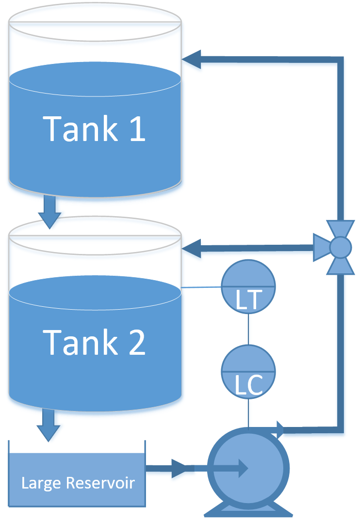
A pump transports water to tank 1 where it drains to tank 2. Both tanks have an opening at the bottom that allows liquid to flow out. A valve is used to divert pumped liquid into tank 1 (valve position=0), into tank 2 (valve position=1) or fractionally into both (valve position 0-1). The valve position is not available to the controller as a measurement and is considered a disturbance to the process. Only the level of tank 2 (bottom tank) is available as a measured value. The pump rate can be manipulated between 0 and 1. The pump has a maximum rate of change of 0.1 every second.

For control you can use linear or nonlinear model predictive control. For estimation, you can use moving horizon estimation (MHE) or simple bias updating. The simplest option is linear MPC with bias updating. The following is a linear second order model that approximates the level dynamics.
$$\tau_{1} \frac{h_1}{dt} = -h_1 + K_1 \, p$$ $$\tau_{2} \frac{h_2}{dt} = -h_2 + K_2 \, h_1$$
where 1 and 2 refer to the tanks, `\tau_1=18.4` and `\tau_2=24.4` are time constants, `K_1=1.3` and `K_2=1.0` are gains, `h_1` and `h_2` are liquid level heights, and p is the pump flow between 0 and 1.
Python (GEKKO Solution)
import matplotlib.pyplot as plt
from scipy.integrate import odeint
import csv
from gekko import GEKKO
# create MPC with GEKKO
m = GEKKO()
m.time = [0,1,2,4,8,12,16,20]
# empirical constants
Kp_h1 = 1.3
tau_h1 = 18.4
Kp_h2 = 1
tau_h2 = 24.4
# manipulated variable
p = m.MV(value=0,lb=1e-5,ub=1)
p.STATUS = 1
p.DCOST = 0.01
p.FSTATUS = 0
# unmeasured state
h1 = m.Var(value=0.0)
# controlled variable
h2 = m.CV(value=0.0)
h2.STATUS = 1
h2.FSTATUS = 1
h2.TAU = 20
h2.TR_INIT = 1
# equations
m.Equation(tau_h1*h1.dt()==-h1 + Kp_h1*p)
m.Equation(tau_h2*h2.dt()==-h2 + Kp_h2*h1)
# options
m.options.IMODE = 6
m.options.CV_TYPE = 2
# simulated system (for measurements)
def tank(levels,t,pump,valve):
h1 = max(1.0e-10,levels[0])
h2 = max(1.0e-10,levels[1])
c1 = 0.08 # inlet valve coefficient
c2 = 0.04 # tank outlet coefficient
dhdt1 = c1 * (1.0-valve) * pump - c2 * np.sqrt(h1)
dhdt2 = c1 * valve * pump + c2 * np.sqrt(h1) - c2 * np.sqrt(h2)
if h1>=1.0 and dhdt1>0.0:
dhdt1 = 0
if h2>=1.0 and dhdt2>0.0:
dhdt2 = 0
dhdt = [dhdt1,dhdt2]
return dhdt
# Initial conditions (levels)
h0 = [0,0]
# Time points to report the solution
tf = 400
t = np.linspace(0,tf,tf+1)
# Set point
sp = np.zeros(tf+1)
sp[5:100] = 0.5
sp[100:200] = 0.8
sp[200:300] = 0.2
sp[300:] = 0.5
# Inputs that can be adjusted
pump = np.zeros(tf+1)
# Disturbance
valve = 0.0
# Record the solution
y = np.zeros((tf+1,2))
y[0,:] = h0
# Create plot
plt.figure(figsize=(10,7))
plt.ion()
plt.show()
# Simulate the tank step test
for i in range(1,tf):
#########################
# MPC ###################
#########################
# measured height
h2.MEAS = y[i,1]
# set point deadband
h2.SPHI = sp[i]+0.01
h2.SPLO = sp[i]-0.01
h2.SP = sp[i]
# solve MPC
m.solve(disp=False)
# retrieve 1st pump new value
pump[i] = p.NEWVAL
#########################
# System ################
#########################
# Specify the pump and valve
inputs = (pump[i],valve)
# Integrate the model
h = odeint(tank,h0,[0,1],inputs)
# Record the result
y[i+1,:] = h[-1,:]
# Reset the initial condition
h0 = h[-1,:]
# update plot every 5 cycles
if (i%5==3):
plt.clf()
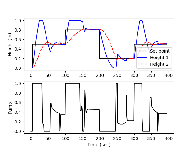
plt.subplot(2,1,1)
plt.plot(t[0:i],sp[0:i],'k-')
plt.plot(t[0:i],y[0:i,0],'b-')
plt.plot(t[0:i],y[0:i,1],'r--')
plt.ylabel('Height (m)')
plt.legend(['Set point','Height 1','Height 2'])
plt.subplot(2,1,2)
plt.plot(t[0:i],pump[0:i],'k-')
plt.ylabel('Pump')
plt.xlabel('Time (sec)')
plt.draw()
plt.pause(0.01)
# Construct and save data file
data = np.vstack((t,pump))
data = np.hstack((np.transpose(data),y))
np.savetxt('data.txt',data,delimiter=',')
Python (GEKKO Animated Solution)
import matplotlib.pyplot as plt
from scipy.integrate import odeint
from gekko import GEKKO
from matplotlib.widgets import Button
import time
tf = 200
t_span = np.linspace(0, tf, tf + 1)
valve = 0.0
# Setpoint trajectory
sp = np.ones(tf + 1) *0.5
sp[int(tf/2):] = np.random.choice([0.2, 0.3, 0.4, 0.6, 0.7, 0.8])
# Create plots
scale = 0.5
fig, axs = plt.subplots(3, 2, figsize=(16*scale, 9*scale), sharey='row', gridspec_kw={'width_ratios': [1, 2]})
# Initialize bar plots
tank_1_bar, = axs[0, 0].bar(x = 0, height = 0, width = 1.0, color = 'b', label='Tank 1 Level')
tank_2_bar, = axs[1, 0].bar(x = 0, height = 0, width = 1.0, color = 'b', label='Tank 2 Level')
pump_speed, = axs[2, 0].bar(x = 0, height = 0.5, width = 1.0, facecolor = 'none', edgecolor = 'black', label='Pump speed')
# Initialize line plots
line_y1, = axs[0, 1].plot([], [], 'b-', label='Manual')
line_y1_gekko, = axs[0, 1].plot([], [], 'b--', label='GEKKO MPC')
line_y2, = axs[1, 1].plot([], [], 'r-', label='Manual')
line_y2_gekko, = axs[1, 1].plot([], [], 'r--', label='GEKKO MPC')
line_sp, = axs[1, 1].plot([], [], 'k-', label='Setpoint')
line_pump, = axs[2, 1].plot([], [], 'g-', label='Manual')
line_pump_gekko, = axs[2, 1].plot([], [], 'g--', label='GEKKO MPC')
# Set axes ranges and labels
axs[0, 1].legend()
axs[1, 1].legend()
axs[2, 1].legend()
axs[0, 0].set_ylabel('Tank 1 level')
axs[0, 0].set_xlim(-0.5,0.5)
axs[0, 0].set_ylim(-0.1,1.1)
axs[0, 0].set_title = 'Tank 1 level'
axs[1, 0].set_ylabel('Tank 2 level')
axs[1, 0].set_xlim(-0.5,0.5)
axs[1, 0].set_ylim(-0.1,1.1)
axs[2, 0].set_ylabel('Pump speed')
axs[2, 0].set_xlim(-0.5,0.5)
axs[2, 0].set_ylim(-0.1,1.6)
axs[0, 1].set_xlim(0,tf)
axs[1, 1].set_xlim(0,tf)
axs[2, 1].set_xlim(0,tf)
axs[2, 1].set_xlabel('Time')
# Show the tank and pump limit lines
axs[0,0].plot([-0.5, 0.5], [1.0, 1.0], 'k:')
axs[1,0].plot([-0.5, 0.5], [1.0, 1.0], 'k:')
axs[2,0].plot([-0.5, 0.5], [1.5, 1.5], 'k:')
axs[0,1].plot([0, tf], [1.0, 1.0], 'k:')
axs[1,1].plot([0, tf], [1.0, 1.0], 'k:')
axs[2,1].plot([0, tf], [1.5, 1.5], 'k:')
# Create button axes
ax_increase = plt.axes([0.8, 0.02, 0.1, 0.04])
ax_decrease = plt.axes([0.7, 0.02, 0.1, 0.04])
# Create buttons
btn_increase = Button(ax_increase, 'Pump +0.05')
btn_decrease = Button(ax_decrease, 'Pump -0.05')
plt.ion()
plt.show()
# Simulated system (for measurements)
def tank(levels, t, pump, valve):
h1 = max(1.0e-10, levels[0])
h2 = max(1.0e-10, levels[1])
c1 = 0.08 # inlet valve coefficient
c2 = 0.04 # tank outlet coefficient
dhdt1 = c1 * (1.0 - valve) * pump - c2 * np.sqrt(h1)
dhdt2 = c1 * valve * pump + c2 * np.sqrt(h1) - c2 * np.sqrt(h2)
if h1 >= 1.0 and dhdt1 > 0.0:
dhdt1 = 0
if h2 >= 1.0 and dhdt2 > 0.0:
dhdt2 = 0
return [dhdt1, dhdt2]
def sim():
# Manual simulation loop
current_i = 0
# Initial conditions
h0 = [0, 0]
# Record the solution
y = np.zeros((tf + 1, 2))
y[0, :] = h0
# Initial pump values
current_pump = 0.5 # Initial pump value
pump = np.ones(tf + 1) * current_pump # Initialize pump array
# Button callback functions
def increase_pump(event):
nonlocal current_pump, pump, current_i
current_pump = min(current_pump + 0.05, 1.5)
pump[current_i:] = current_pump
def decrease_pump(event):
nonlocal current_pump, pump, current_i
current_pump = max(current_pump - 0.05, 0.0)
pump[current_i:] = current_pump
# Connect buttons
btn_increase.on_clicked(increase_pump)
btn_decrease.on_clicked(decrease_pump)
for i in range(tf):
current_i = i
# Integrate the model
inputs = (pump[i], valve)
h = odeint(tank, y[i, :], [0, 1], inputs)
# Record the result
y[i + 1, :] = h[-1, :]
# Update bar plot data
tank_1_bar.set_height(y[i + 1, 0])
tank_2_bar.set_height(y[i + 1, 1])
pump_speed.set_height(pump[i])
# Change the bar colors if the tanks overflow
if y[i + 1, 0] < 1.0:
tank_1_bar.set_color('b')
else:
tank_1_bar.set_color('r')
if y[i + 1, 1] < 1.0:
tank_2_bar.set_color('b')
else:
tank_2_bar.set_color('r')
# Update line data
line_sp.set_data(t_span[:i + 1], sp[:i + 1])
line_y1.set_data(t_span[:i + 1], y[:i + 1, 0])
line_y2.set_data(t_span[:i + 1], y[:i + 1, 1])
line_pump.set_data(t_span[:i + 1], pump[:i + 1])
plt.pause(0.015)
# Allow some time adjust the figure area
if i == 0:
plt.pause(5)
## GEKKO MPC Solution ##
# Reset initial conditions
h0 = [0,0]
y = np.zeros((tf+1,2))
y[0,:] = h0
pump = np.zeros(tf+1)
# create MPC with GEKKO
m = GEKKO(remote = False)
m.time = [0, 2, 4, 8, 10, 20]
# empirical constants
Kp_h1 = 1.4
tau_h1 = 18.4
Kp_h2 = 1
tau_h2 = 24.4
# manipulated variable (pump)
p = m.MV(value=0.5,lb=1e-5,ub=1.5)
p.STATUS = 1
p.DCOST = 0.01
p.FSTATUS = 0
# unmeasured state
h1 = m.Var(value=0.0, ub = 0.90)
# controlled variable
h2 = m.CV(value=0.0)
h2.STATUS = 1
h2.FSTATUS = 1
h2.TAU = 20
h2.TR_INIT = 1
# equations
m.Equation(tau_h1*h1.dt()==-h1 + Kp_h1*p)
m.Equation(tau_h2*h2.dt()==-h2 + Kp_h2*h1)
# options
m.options.IMODE = 6
m.options.CV_TYPE = 2
m.options.MV_STEP_HOR = 1
# GEKKO simulation loop
current_i = 0
for i in range(tf):
current_i = i
#########################
# MPC ###################
#########################
# measured height
h2.MEAS = y[i,1]
# set point deadband
h2.SPHI = sp[i]+0.01
h2.SPLO = sp[i]-0.01
h2.SP = sp[i]
# solve MPC
m.solve(disp=False)
# retrieve 1st pump new value
pump[i] = p.NEWVAL
#########################
# System ################
#########################
# Specify the pump and valve
inputs = (pump[i],valve)
# Integrate the model
h = odeint(tank,h0,[0,1],inputs)
# Record the result
y[i+1,:] = h[-1,:]
# Reset the initial condition
h0 = h[-1,:]
# Update bar plot data
tank_1_bar.set_height(y[i + 1, 0])
tank_2_bar.set_height(y[i + 1, 1])
# Change the bar colors if the tanks overflow
if y[i + 1, 0] < 1.0:
tank_1_bar.set_color('b')
else:
tank_1_bar.set_color('r')
if y[i + 1, 1] < 1.0:
tank_2_bar.set_color('b')
else:
tank_2_bar.set_color('r')
pump_speed.set_height(pump[i])
# Update line data
line_y1_gekko.set_data(t_span[:i], y[:i, 0])
line_y2_gekko.set_data(t_span[:i], y[:i, 1])
line_pump_gekko.set_data(t_span[:i], pump[:i])
plt.pause(0.01)
run_sim = True
while run_sim:
sim()
z = input('Run again (Y/N)?')
run_sim = True if z.upper() == 'Y' else False
if run_sim:
# Reset bar plots
tank_1_bar.set_height(0)
tank_2_bar.set_height(0)
pump_speed.set_height(0.5)
# Reset line plots
line_y1.set_data([], [])
line_y1_gekko.set_data([], [])
line_y2.set_data([], [])
line_y2_gekko.set_data([], [])
line_sp.set_data([], [])
line_pump.set_data([], [])
line_pump_gekko.set_data([], [])
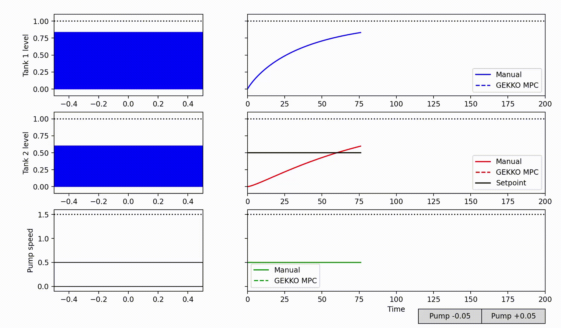
The animated MPC solution begins with manual control and then switches to MPC for comparison. Thanks to Vincent Roos for providing the animated MPC solution.