Dynamics and Control

Time delay is a shift in the effect of an input on an output dynamic response. A first-order linear system with time delay is:

$$\tau_p \frac{dy(t)}{dt} = -y(t) + K_p u\left(t-\theta_p\right)$$

has variables y(t) and u(t) and three unknown parameters with

$$K_p \quad \mathrm{= Process \; gain}$$

$$\tau_p \quad \mathrm{= Process \; time \; constant}$$

$$\theta_p \quad \mathrm{= Process \; dead \; time}$$

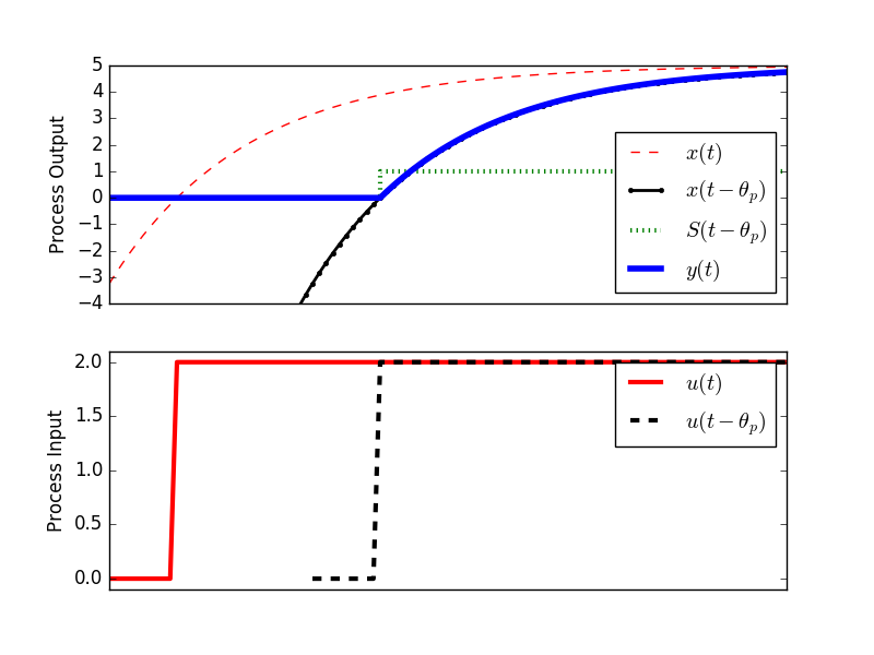
The time delay `\theta_p` is expressed as a time shift in the input variable u(t).

$$u\left(t-\theta_p\right)$$

$$y(t \lt \theta_p) = y(0)$$

$$y(t \ge \theta_p) = \left( e^{-\left(t - \theta_p \right) / \tau_p}\right) y(0) + \left( 1 - e^{-\left(t - \theta_p \right) / \tau_p} \right) K_p \Delta u $$

For a step change `\Delta u`, the analytical solution for a first-order linear system without time delay (x(t) = y(t) with `theta_p=0`)

$$\tau_p \frac{dx(t)}{dt} = -y(t) + K_p u\left(t\right)$$

is

$$x(t) = K_p \left(1-\exp\left(\frac{-t}{\tau_p}\right)\right) \Delta u$$

With dead-time, the solution becomes:

$$y(t) = x \left( t-\theta_p \right) S \left( t-\theta_p \right)$$

$$\quad = K_p \left( 1- \exp\left(-\frac{ t-\theta_p } { \tau_p } \right) \right) \, \Delta u \, S \left( t-\theta_p \right) $$

where

$$S\left(t-\theta_p\right)$$

is a step function that changes from zero to one at `t=theta_p`.

Analytic Solution Derivation with Laplace Transforms