Linear Programming with Python
 |  |  |  |
|---|
Optimization deals with selecting the best option among a number of possible choices that are feasible or don't violate constraints. Python can be used to optimize parameters in a model to best fit data, increase profitability of a potential engineering design, or meet some other type of objective that can be described mathematically with variables and equations.
Mathematical optimization problems may include equality constraints (e.g. =), inequality constraints (e.g. <, <=, >, >=), objective functions, algebraic equations, differential equations, continuous variables, discrete or integer variables, etc. A general statement of an optimization problem with nonlinear objectives or constraints is given by the following:
$$\begin{align}\mathrm{minimize} \quad & c\,x \\ \mathrm{subject\;to}\quad & A \, x=b \\ & A \, x>b \end{align}$$
Two popular numerical methods for solving linear programming problems are the Simplex method and Interior Point method.
Exercise: Soft Drink Production
A simple production planning problem is given by the use of two ingredients A and B that produce products 1 and 2. The available supply is A=30 units and B=44 units. For production it requires:
- 3 units of A and 8 units of B to produce Product 1
- 6 units of A and 4 units of B to produce Product 2
There are at most 5 units of Product 1 and 4 units of Product 2. Product 1 can be sold for 100 and Product 2 can be sold for 125. The objective is to maximize the profit for this production problem.
For this problem determine:
- A potential feasible solution
- Identify the constraints on the contour plot
- Mark the set of feasible solutions on the contour plot
- Identify the minimum objective feasible solution
- Identify the maximum objective feasible solution
- Use a solver to find a solution
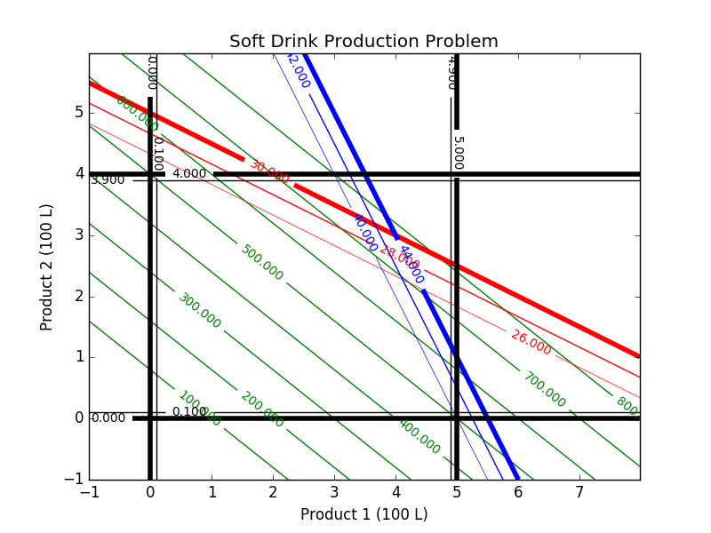
A contour plot can be used to explore the optimal solution. In this case, the black lines indicate the upper and lower bounds on the production of 1 and 2. In this case, the production of 1 must be greater than 0 but less than 5. The production of 2 must be greater than 0 but less than 4. There are at most 30 units of A and 44 units of B ingredients that are available to produce products 1 and 2.
Solution
Method 1: Equations and Objective
Using equations and an objective function is good for small problems because it is a readable optimization problem and is thereby easy to modify.
Python (Gekko)
m = GEKKO()
x1 = m.Var(lb=0, ub=5) # Product 1
x2 = m.Var(lb=0, ub=4) # Product 2
m.Maximize(100*x1+125*x2) # Profit function
m.Equation(3*x1+6*x2<=30) # Units of A
m.Equation(8*x1+4*x2<=44) # Units of B
m.solve(disp=False)
p1 = x1.value[0]; p2 = x2.value[0]
print ('Product 1 (x1): ' + str(p1))
print ('Product 2 (x2): ' + str(p2))
print ('Profit : ' + str(100*p1+125*p2))
MATLAB (Gekko)
x1 = m.Var(pyargs('lb',0,'ub',5)); % Product 1
x2 = m.Var(pyargs('lb',0,'ub',4)); % Product 2
m.Maximize(100*x1+125*x2); % Profit function
m.Equation(3*x1+6*x2<=30); % Units of A
m.Equation(8*x1+4*x2<=44); % Units of B
m.solve(pyargs('disp',false));
p1 = x1.VALUE{1};
p2 = x2.VALUE{1};
disp(['Product 1 (x1): ', num2str(p1)])
disp(['Product 2 (x2): ', num2str(p2)])
disp(['Profit : ', num2str(100*p1+125*p2)])
Method 2a: Dense Matrices (Scipy linprog)
For large-scale problems, a matrix forms is best because it simplifies the problem description and improves the speed of solution. Scipy.optimize.linprog is one of the available packages to solve Linear programming problems. Another good linear and mixed integer programming Python package is Pulp with interfaces to dedicate mixed integer linear programming solvers.
from scipy.optimize import linprog
c = [-100, -125]
A = [[3, 6], [8, 4]]
b = [30, 44]
x0_bounds = (0, 5)
x1_bounds = (0, 4)
res = linprog(c, A_ub=A, b_ub=b, \
bounds=(x0_bounds, x1_bounds),
options={"disp": True})
print(res)
Method 2b: Dense Matrices (Gekko)
Dense matrix form is also available in Gekko. In this case, two model functions qobj (quadratic objective) and axb (Ax<b) objects are used to create the model. Integer variables for discrete optimization are possible with the APOPT solver (option 1) when the variable is specified with integer=True. See Model Building Functions in the Gekko documentation.
m = GEKKO(remote=False)
c = [100, 125]
A = [[3, 6], [8, 4]]
b = [30, 44]
x = m.qobj(c,otype='max')
m.axb(A,b,x=x,etype='<')
x[0].lower=0; x[0].upper=5
x[1].lower=0; x[1].upper=4
m.options.solver = 1
m.solve(disp=True)
print ('Product 1 (x1): ' + str(x[0].value[0]))
print ('Product 2 (x2): ' + str(x[1].value[0]))
print ('Profit : ' + str(-m.options.objfcnval))
Method 3: Sparse Matrices (Gekko)
Sparse matrices are faster and use less memory for very large-scale problems with many zeros in A, b, and c.
import numpy as np
from gekko import GEKKO
m = GEKKO(remote=False)
# [[row indices],[column indices],[values]]
A_sparse = [[1,1,2,2],[1,2,1,2],[3,6,8,4]]
# [[row indices],[values]]
b_sparse = [[1,2],[30,44]]
x = m.axb(A_sparse,b_sparse,etype='<',sparse=True)
# [[row indices],[values]]
c_sparse = [[1,2],[100,125]]
m.qobj(c_sparse,x=x,otype='max',sparse=True)
x[0].lower=0; x[0].upper=5
x[1].lower=0; x[1].upper=4
m.solve(disp=True)
print ('Product 1 (x1): ' + str(x[0].value[0]))
print ('Product 2 (x2): ' + str(x[1].value[0]))
print ('Profit : ' + str(-m.options.objfcnval))
Contour Plot
Below are the source files for generating the contour plots in Python. The linear program is solved with the APM model through a web-service while the contour plot is generated with the Python package Matplotlib.
m = GEKKO()
# variables
x1 = m.Var(value=0 , lb=0 , ub=5 , name='x1') # Product 1
x2 = m.Var(value=0 , lb=0 , ub=4 , name='x2') # Product 2
profit = m.Var(value=1 , name='profit')
# profit function
m.Obj(-profit)
m.Equation(profit==100*x1+125*x2)
m.Equation(3*x1+6*x2<=30)
m.Equation(8*x1+4*x2<=44)
m.solve()
print ('')
print ('--- Results of the Optimization Problem ---')
print ('Product 1 (x1): ' + str(x1[0]))
print ('Product 2 (x2): ' + str(x2[0]))
print ('Profit: ' + str(profit[0]))
## Generate a contour plot
# Import some other libraries that we'll need
# matplotlib and numpy packages must also be installed
import matplotlib
import numpy as np
import matplotlib.pyplot as plt
# Design variables at mesh points
x = np.arange(-1.0, 8.0, 0.02)
y = np.arange(-1.0, 6.0, 0.02)
x1, x2 = np.meshgrid(x,y)
# Equations and Constraints
profit = 100.0 * x1 + 125.0 * x2
A_usage = 3.0 * x1 + 6.0 * x2
B_usage = 8.0 * x1 + 4.0 * x2
# Create a contour plot
plt.figure()
# Weight contours
lines = np.linspace(100.0,800.0,8)
CS = plt.contour(x1,x2,profit,lines,colors='g')
plt.clabel(CS, inline=1, fontsize=10)
# A usage < 30
CS = plt.contour(x1,x2,A_usage,[26.0, 28.0, 30.0],colors='r',linewidths=[0.5,1.0,4.0])
plt.clabel(CS, inline=1, fontsize=10)
# B usage < 44
CS = plt.contour(x1, x2,B_usage,[40.0,42.0,44.0],colors='b',linewidths=[0.5,1.0,4.0])
plt.clabel(CS, inline=1, fontsize=10)
# Container for 0 <= Product 1 <= 500 L
CS = plt.contour(x1, x2,x1 ,[0.0, 0.1, 4.9, 5.0],colors='k',linewidths=[4.0,1.0,1.0,4.0])
plt.clabel(CS, inline=1, fontsize=10)
# Container for 0 <= Product 2 <= 400 L
CS = plt.contour(x1, x2,x2 ,[0.0, 0.1, 3.9, 4.0],colors='k',linewidths=[4.0,1.0,1.0,4.0])
plt.clabel(CS, inline=1, fontsize=10)
# Add some labels
plt.title('Soft Drink Production Problem')
plt.xlabel('Product 1 (100 L)')
plt.ylabel('Product 2 (100 L)')
# Save the figure as a PNG
plt.savefig('contour.png')
# Show the plots
plt.show()
Practice Problem
Solve the Linear Programming problem.
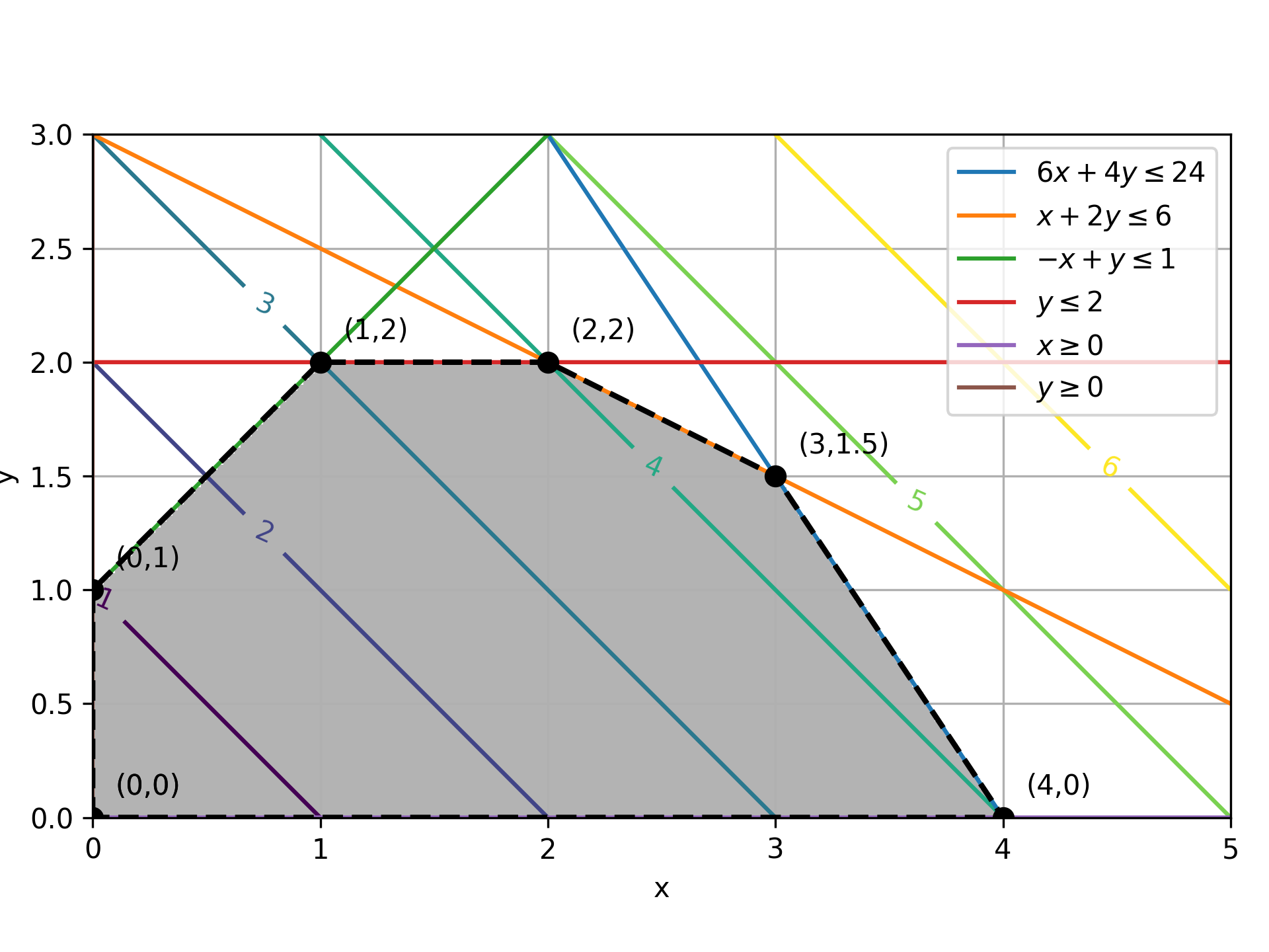
$$\begin{align}\mathrm{maximize} \quad & x+y \\ \mathrm{subject\;to}\quad & 6x+4y\le24 \\ & x+2y\le6 \\ &-x+y\le1 \\ & y\le2 \\ & x\ge0 \\ & y\ge0 \end{align}$$
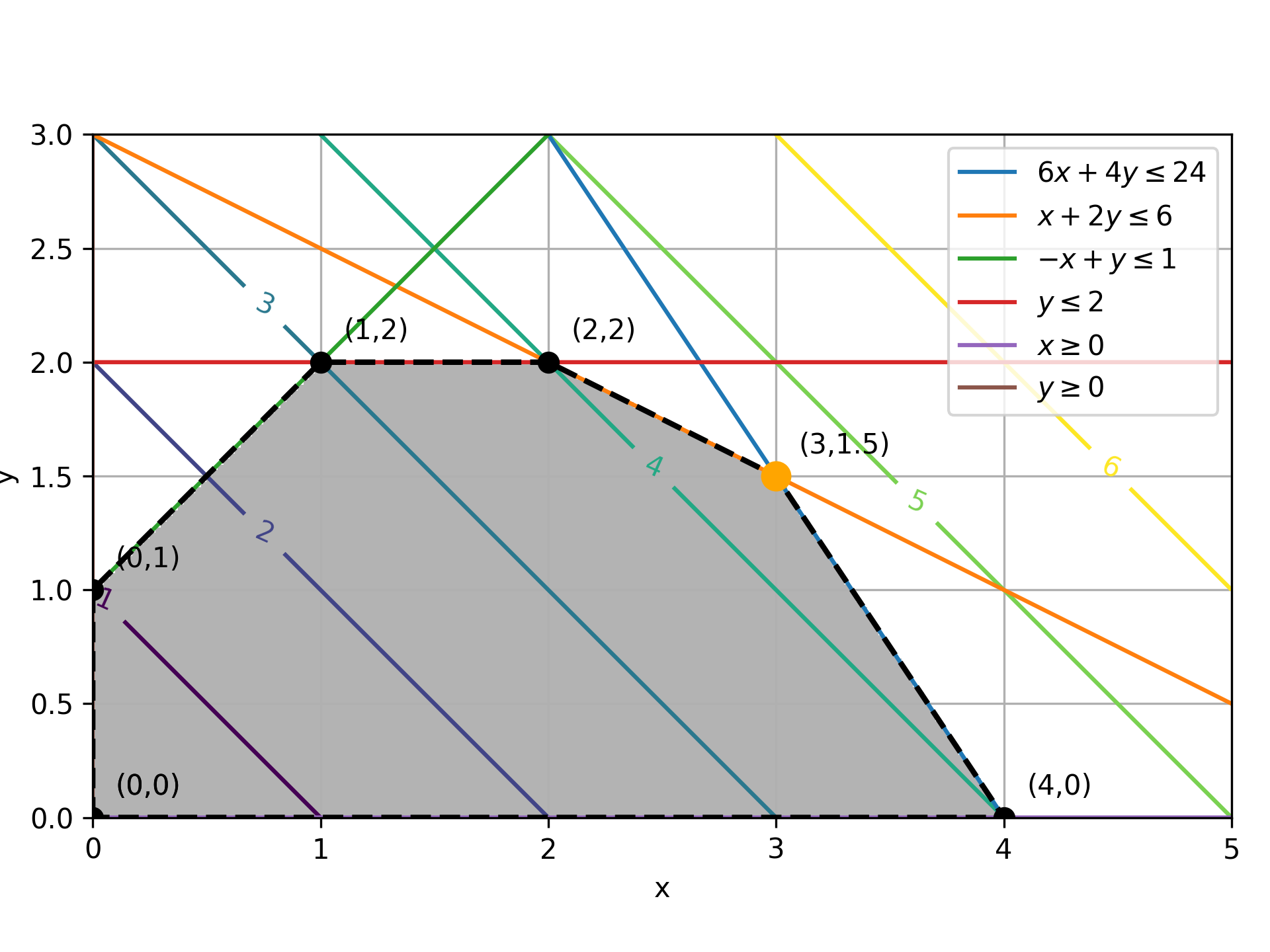
A graphical representation of the constraints and objective is shown in the figure below. The contour lines are the objective and the vertices are labeled. Linear programming solutions are found at vertices (intersection of constraints).
The optimal solution is shown as an orange dot at (3,1.5) with a maximized objective function of 4.5. The optimal solution is at the intersection of two constraints.
import matplotlib.pyplot as plt
from gekko import GEKKO
# solve LP
m = GEKKO(remote=False)
x,y = m.Array(m.Var,2,lb=0)
m.Equations([6*x+4*y<=24,x+2*y<=6,-x+y<=1,y<=2])
m.Maximize(x+y)
m.solve(disp=False)
xopt = x.value[0]; yopt = y.value[0]
# visualize solution
g = np.linspace(0,5,200)
x,y = np.meshgrid(g,g)
obj = x+y
plt.imshow(((6*x+4*y<=24)&(x+2*y<=6)&(-x+y<=1)&(y<=2)&(x>=0)&(y>=0)).astype(int),
extent=(x.min(),x.max(),y.min(),y.max()),origin='lower',cmap='Greys',alpha=0.3);
# plot constraints
x0 = np.linspace(0, 5, 2000)
y0 = 6-1.5*x0 # 6*x+4*y<=24
y1 = 3-0.5*x0 # x+2*y<=6
y2 = 1+x0 # -x+y<=1
y3 = (x0*0) + 2 # y <= 2
y4 = x0*0 # x >= 0
plt.plot(x0, y0, label=r'$6x+4y\leq24$')
plt.plot(x0, y1, label=r'$x+2y\leq6$')
plt.plot(x0, y2, label=r'$-x+y\leq1$')
plt.plot(x0, 2*np.ones_like(x0), label=r'$y\leq2$')
plt.plot(x0, y4, label=r'$x\geq0$')
plt.plot([0,0],[0,3], label=r'$y\geq0$')
xv = [0,0,1,2,3,4,0]; yv = [0,1,2,2,1.5,0,0]
plt.plot(xv,yv,'ko--',markersize=7,linewidth=2)
for i in range(len(xv)):
plt.text(xv[i]+0.1,yv[i]+0.1,f'({xv[i]},{yv[i]})')
# objective contours
CS = plt.contour(x,y,obj,np.arange(1,7))
plt.clabel(CS, inline=1, fontsize=10)
# optimal point
plt.plot([xopt],[yopt],marker='o',color='orange',markersize=10)
plt.xlim(0,5); plt.ylim(0,3); plt.grid(); plt.tight_layout()
plt.legend(loc=1); plt.xlabel('x'); plt.ylabel('y')
plt.savefig('plot.png',dpi=300)
plt.show()
Additional Resources