Dynamic Simulation in Python
 |  |  |  |
|---|
A step response is a common evaluation of the dynamics of a simulated system. A linear time invariant (LTI) system can be described equivalently as a transfer function, a state space model, or solved numerically with and ODE integrator. This tutorial shows how to simulate a first and second order system in Python.


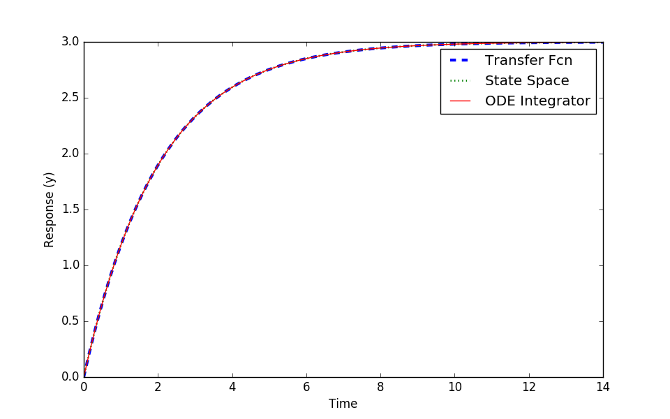
First Order System Simulation
Consider a first order differential equation with constants `K_p=3` and `\tau_p=2`, input `u`, and output response `y`.
$$\tau_p \frac{dy}{dt} = -y + K_p u$$
Three methods to represent this differential equation is as a (1) transfer function, (2) state space model, and (3) semi-explicit differential equation. Source code is included below to simulate a step response in these three forms.
1. Transfer Function
$$\frac{Y(s)}{U(s)} = \frac{K_p}{\tau_p \,s + 1}$$
2. State Space Model
$$\dot x = A x + B u$$
$$y = C x + D u$$
$$A = -\frac{1}{\tau_p} \quad B = \frac{K_p}{\tau_p} \quad C=1 \quad D=0$$
3. Differential Equation
$$\frac{dy}{dt} = -\frac{1}{\tau_p} y + \frac{K_p}{\tau_p} u$$
from scipy import signal
import matplotlib.pyplot as plt
from scipy.integrate import odeint
# Simulate taup * dy/dt = -y + K*u
Kp = 3.0
taup = 2.0
# (1) Transfer Function
num = [Kp]
den = [taup,1]
sys1 = signal.TransferFunction(num,den)
t1,y1 = signal.step(sys1)
# (2) State Space
A = -1.0/taup
B = Kp/taup
C = 1.0
D = 0.0
sys2 = signal.StateSpace(A,B,C,D)
t2,y2 = signal.step(sys2)
# (3) ODE Integrator
def model3(y,t):
u = 1
return (-y + Kp * u)/taup
t3 = np.linspace(0,14,100)
y3 = odeint(model3,0,t3)
plt.figure(1)
plt.plot(t1,y1,'b--',linewidth=3,label='Transfer Fcn')
plt.plot(t2,y2,'g:',linewidth=2,label='State Space')
plt.plot(t3,y3,'r-',linewidth=1,label='ODE Integrator')
plt.xlabel('Time')
plt.ylabel('Response (y)')
plt.legend(loc='best')
plt.show()
Second Order System Simulation
1. Laplace Domain, Transfer Function
$$\frac{Y(s)}{U(s)} = \frac{K_p}{\tau_s^2 s^2 + 2 \zeta \tau_s s + 1}e^{-\theta_p s}$$
2. State Space Form
$$\begin{bmatrix}\dot x_1\\\dot x_2\end{bmatrix} = \begin{bmatrix}0&1\\-\frac{1}{\tau_s^2}&-\frac{2 \zeta}{\tau_s}\end{bmatrix} \begin{bmatrix}x_1\\x_2\end{bmatrix} + \begin{bmatrix}0\\\frac{K_p}{\tau_{s}^2}\end{bmatrix} u\left(t-\theta_p\right)$$
$$y = \begin{bmatrix}1 & 0\end{bmatrix} \begin{bmatrix}x_1\\x_2\end{bmatrix} + \begin{bmatrix}0\end{bmatrix} u$$
3. Second Order Differential Equation
$$\tau_s^2 \frac{d^2y}{dt^2} + 2 \zeta \tau_s \frac{dy}{dt} + y = K_p \, u\left(t-\theta_p \right)$$
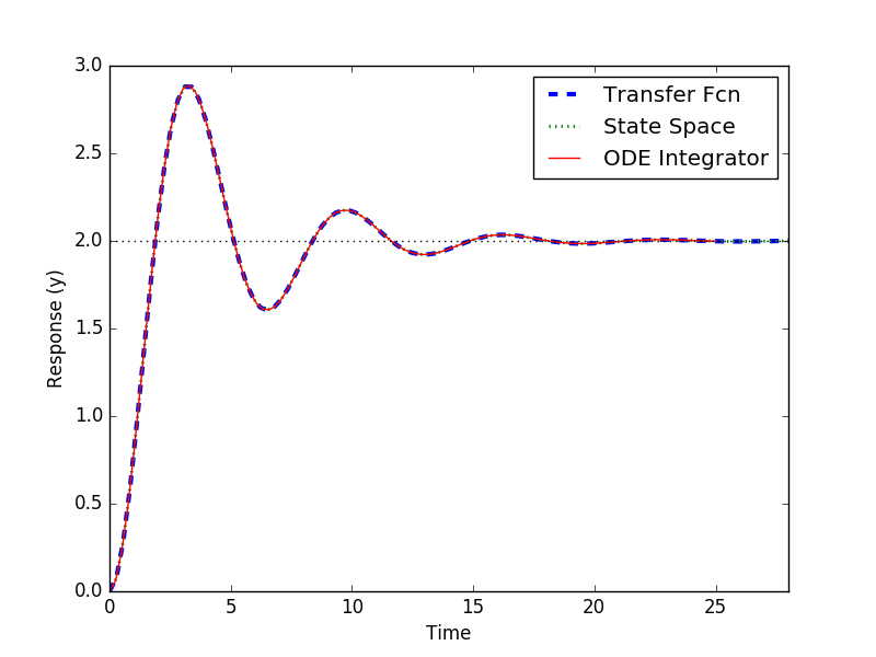
 Kp    = 2.0  # gain
 tau   = 1.0  # time constant
 zeta  = 0.25 # damping factor
 theta = 0.0  # no time delay
from scipy import signal
import matplotlib.pyplot as plt
from scipy.integrate import odeint
# tau * dy2/dt2 + 2*zeta*tau*dy/dt + y = Kp*u
Kp = 2.0 # gain
tau = 1.0 # time constant
zeta = 0.25 # damping factor
theta = 0.0 # no time delay
du = 1.0 # change in u
# (1) Transfer Function
num = [Kp]
den = [tau**2,2*zeta*tau,1]
sys1 = signal.TransferFunction(num,den)
t1,y1 = signal.step(sys1)
# (2) State Space
A = [[0.0,1.0],[-1.0/tau**2,-2.0*zeta/tau]]
B = [[0.0],[Kp/tau**2]]
C = [1.0,0.0]
D = 0.0
sys2 = signal.StateSpace(A,B,C,D)
t2,y2 = signal.step(sys2)
# (3) ODE Integrator
def model3(x,t):
y = x[0]
dydt = x[1]
dy2dt2 = (-2.0*zeta*tau*dydt - y + Kp*du)/tau**2
return [dydt,dy2dt2]
t3 = np.linspace(0,25,100)
x3 = odeint(model3,[0,0],t3)
y3 = x3[:,0]
plt.figure(1)
plt.plot(t1,y1*du,'b--',linewidth=3,label='Transfer Fcn')
plt.plot(t2,y2*du,'g:',linewidth=2,label='State Space')
plt.plot(t3,y3,'r-',linewidth=1,label='ODE Integrator')
y_ss = Kp * du
plt.plot([0,max(t1)],[y_ss,y_ss],'k:')
plt.xlim([0,max(t1)])
plt.xlabel('Time')
plt.ylabel('Response (y)')
plt.legend(loc='best')
plt.savefig('2nd_order.png')
plt.show()
Higher Order Simulation
A simple higher order simulation is the combination of n first order equations. The value of the time constant is 10/n in this example. The first equation is a first order differential expression.
$$\tau \frac{dy_1}{dt} = -y_1 + 1$$
Additional equations are also first order differential expressions for i = 2, n.
$$\tau \frac{dy_i}{dt} = -y_i + y_{i-1}$$