Arduino Temperature PID Control
Obtain PID tuning constants `K_c`, `\tau_I`, and `\tau_D` from IMC correlations. Use the tuning constants for PID control of temperature. Demonstrate step changes in temperature set point and comment on the performance of the Arduino controller using the calculated constants. Tune the controller by adjusting the constants to improve performance. Comment on the difference between IMC tuning constants and the improved tuning constants in terms of rise time, overshoot, decay ratio, heater fluctuations, or other relevant performance criteria.
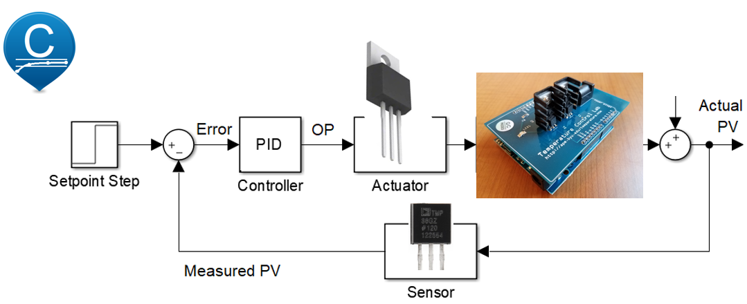
Simulate a PID Controller with one of the models determined from parameter estimation. Below is basic code in Python that demonstrates how to implement a PID controller. On each cycle of the controller, the temperature is measured (a.T1), the PID controller produces a new output (OP=pid(a.T1)), and the PID recommended value for the heater is implemented (a.Q1(OP)). The loop pauses for the 1.0 second to wait until the next sample time.
import time
import numpy as np
from simple_pid import PID
# Connect to Arduino
a = tclab.TCLab()
# Create PID controller
pid = PID(Kp=2,Ki=2/136,Kd=0,\
setpoint=40,sample_time=1.0,output_limits=(0,100))
for i in range(300): # 5 minutes (300 sec)
# pid control
OP = pid(a.T1)
a.Q1(OP)
# print line
print('Heater: ' + str(round(OP,2)) + '%' + \
' T PV: ' + str(a.T1) + 'degC' + \
' T SP: ' + str(pid.setpoint) + 'degC')
# wait for next sample time
time.sleep(pid.sample_time)
It is suggested to tune the controller in simulation before implementing with an Arduino. Tuning on a device that takes 10-20 minutes per test is much slower than running a PID controller in simulation. Once optimized PID tuning values are obtained, demonstrate the performance with the physical control lab.
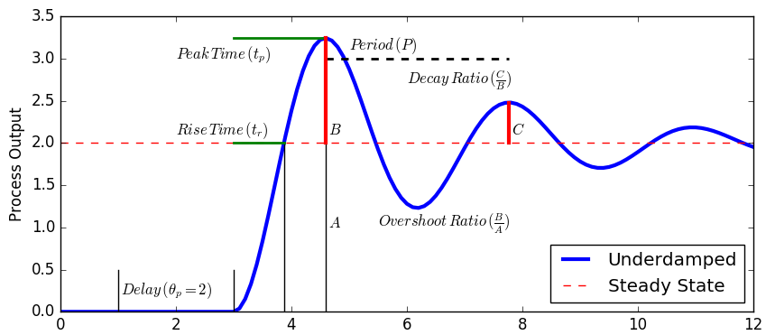
Tune the PID controller to minimize the sum of absolute error and achieve an overshoot ratio less than 10%. Quantify the controller performance in terms of settling time, decay ratio, overshoot ratio, peak time, and rise time.
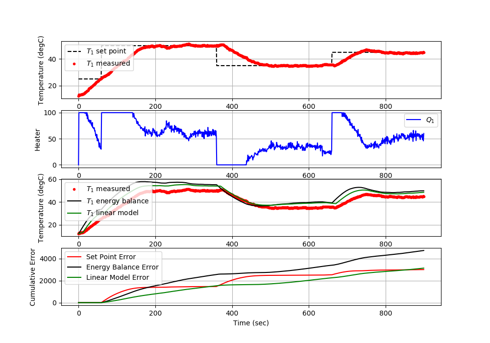
Use the following code to test the models and PID controller.
import numpy as np
import time
import matplotlib.pyplot as plt
from scipy.integrate import odeint
######################################################
# Use this script for evaluating model predictions #
# and PID controller performance for the TCLab #
# Adjust only PID and model sections #
######################################################
######################################################
# PID Controller #
######################################################
# inputs -----------------------------------
# sp = setpoint
# pv = current temperature
# pv_last = prior temperature
# ierr = integral error
# dt = time increment between measurements
# outputs ----------------------------------
# op = output of the PID controller
# P = proportional contribution
# I = integral contribution
# D = derivative contribution
def pid(sp,pv,pv_last,ierr,dt):
Kc = 10.0 # K/%Heater
tauI = 50.0 # sec
tauD = 1.0 # sec
# Parameters in terms of PID coefficients
KP = Kc
KI = Kc/tauI
KD = Kc*tauD
# ubias for controller (initial heater)
op0 = 0
# upper and lower bounds on heater level
ophi = 100
oplo = 0
# calculate the error
error = sp-pv
# calculate the integral error
ierr = ierr + KI * error * dt
# calculate the measurement derivative
dpv = (pv - pv_last) / dt
# calculate the PID output
P = KP * error
I = ierr
D = -KD * dpv
op = op0 + P + I + D
# implement anti-reset windup
if op < oplo or op > ophi:
I = I - KI * error * dt
# clip output
op = max(oplo,min(ophi,op))
# return the controller output and PID terms
return [op,P,I,D]
######################################################
# FOPDT model #
######################################################
Kp = 0.5 # degC/%
tauP = 120.0 # seconds
thetaP = 10 # seconds (integer)
Tss = 23 # degC (ambient temperature)
Qss = 0 # % heater
######################################################
# Energy balance model #
######################################################
def heat(x,t,Q):
# Parameters
Ta = 23 + 273.15 # K
U = 10.0 # W/m^2-K
m = 4.0/1000.0 # kg
Cp = 0.5 * 1000.0 # J/kg-K
A = 12.0 / 100.0**2 # Area in m^2
alpha = 0.01 # W / % heater
eps = 0.9 # Emissivity
sigma = 5.67e-8 # Stefan-Boltzman
# Temperature State
T = x[0]
# Nonlinear Energy Balance
dTdt = (1.0/(m*Cp))*(U*A*(Ta-T) \
+ eps * sigma * A * (Ta**4 - T**4) \
+ alpha*Q)
return dTdt
######################################################
# Do not adjust anything below this point #
######################################################
# Connect to Arduino
a = tclab.TCLab()
# Turn LED on
print('LED On')
a.LED(100)
# Run time in minutes
run_time = 15.0
# Number of cycles
loops = int(60.0*run_time)
tm = np.zeros(loops)
# Temperature
# set point (degC)
Tsp1 = np.ones(loops) * 25.0
Tsp1[60:] = 50.0
Tsp1[360:] = 30.0
Tsp1[660:] = 40.0
T1 = np.ones(loops) * a.T1 # measured T (degC)
error_sp = np.zeros(loops)
Tsp2 = np.ones(loops) * 23.0 # set point (degC)
T2 = np.ones(loops) * a.T2 # measured T (degC)
# Predictions
Tp = np.ones(loops) * a.T1
error_eb = np.zeros(loops)
Tpl = np.ones(loops) * a.T1
error_fopdt = np.zeros(loops)
# impulse tests (0 - 100%)
Q1 = np.ones(loops) * 0.0
Q2 = np.ones(loops) * 0.0
print('Running Main Loop. Ctrl-C to end.')
print(' Time SP PV Q1 = P + I + D')
print(('{:6.1f} {:6.2f} {:6.2f} ' + \
'{:6.2f} {:6.2f} {:6.2f} {:6.2f}').format( \
tm[0],Tsp1[0],T1[0], \
Q1[0],0.0,0.0,0.0))
# Create plot
plt.figure(figsize=(10,7))
plt.ion()
plt.show()
# Main Loop
start_time = time.time()
prev_time = start_time
# Integral error
ierr = 0.0
try:
for i in range(1,loops):
# Sleep time
sleep_max = 1.0
sleep = sleep_max - (time.time() - prev_time)
if sleep>=0.01:
time.sleep(sleep-0.01)
else:
time.sleep(0.01)
# Record time and change in time
t = time.time()
dt = t - prev_time
prev_time = t
tm[i] = t - start_time
# Read temperatures in Kelvin
T1[i] = a.T1
T2[i] = a.T2
# Simulate one time step with Energy Balance
Tnext = odeint(heat,Tp[i-1]+273.15,[0,dt],args=(Q1[i-1],))
Tp[i] = Tnext[1]-273.15
# Simulate one time step with linear FOPDT model
z = np.exp(-dt/tauP)
Tpl[i] = (Tpl[i-1]-Tss) * z \
+ (Q1[max(0,i-int(thetaP)-1)]-Qss)*(1-z)*Kp \
+ Tss
# Calculate PID output
[Q1[i],P,ierr,D] = pid(Tsp1[i],T1[i],T1[i-1],ierr,dt)
# Start setpoint error accumulation after 1 minute (60 seconds)
if i>=60:
error_eb[i] = error_eb[i-1] + abs(Tp[i]-T1[i])
error_fopdt[i] = error_fopdt[i-1] + abs(Tpl[i]-T1[i])
error_sp[i] = error_sp[i-1] + abs(Tsp1[i]-T1[i])
# Write output (0-100)
a.Q1(Q1[i])
a.Q2(0.0)
# Print line of data
print(('{:6.1f} {:6.2f} {:6.2f} ' + \
'{:6.2f} {:6.2f} {:6.2f} {:6.2f}').format( \
tm[i],Tsp1[i],T1[i], \
Q1[i],P,ierr,D))
# Plot
plt.clf()
ax=plt.subplot(4,1,1)
ax.grid()
plt.plot(tm[0:i],T1[0:i],'r.',label=r'$T_1$ measured')
plt.plot(tm[0:i],Tsp1[0:i],'k--',label=r'$T_1$ set point')
plt.ylabel('Temperature (degC)')
plt.legend(loc=2)
ax=plt.subplot(4,1,2)
ax.grid()
plt.plot(tm[0:i],Q1[0:i],'b-',label=r'$Q_1$')
plt.ylabel('Heater')
plt.legend(loc='best')
ax=plt.subplot(4,1,3)
ax.grid()
plt.plot(tm[0:i],T1[0:i],'r.',label=r'$T_1$ measured')
plt.plot(tm[0:i],Tp[0:i],'k-',label=r'$T_1$ energy balance')
plt.plot(tm[0:i],Tpl[0:i],'g-',label=r'$T_1$ linear model')
plt.ylabel('Temperature (degC)')
plt.legend(loc=2)
ax=plt.subplot(4,1,4)
ax.grid()
plt.plot(tm[0:i],error_sp[0:i],'r-',label='Set Point Error')
plt.plot(tm[0:i],error_eb[0:i],'k-',label='Energy Balance Error')
plt.plot(tm[0:i],error_fopdt[0:i],'g-',label='Linear Model Error')
plt.ylabel('Cumulative Error')
plt.legend(loc='best')
plt.xlabel('Time (sec)')
plt.draw()
plt.pause(0.05)
# Turn off heaters
a.Q1(0)
a.Q2(0)
# Save figure
plt.savefig('test_PID.png')
# Allow user to end loop with Ctrl-C
except KeyboardInterrupt:
# Disconnect from Arduino
a.Q1(0)
a.Q2(0)
print('Shutting down')
a.close()
plt.savefig('test_PID.png')
# Make sure serial connection still closes when there's an error
except:
# Disconnect from Arduino
a.Q1(0)
a.Q2(0)
print('Error: Shutting down')
a.close()
plt.savefig('test_PID.png')
raise
Return to Temperature Control Lab Overview