Parameter Regression with Arduino Data
The objective of this activity is to fit empirical and physics-based predictions to the data for a two heater model of the temperature control lab. Select parameters are adjusted to minimize the sum of squared errors (SSE) or the integral absolute error (IAE) between the model predicted values and the measured values.
$$IAE_{model} = \sum_{i=0}^n \left| T_{1,meas,i} - T_{1,pred,i} \right| + \left| T_{2,meas,i} - T_{2,pred,i} \right|$$
Use an optimizer to adjust the parameters and achieve alignment between the model and the measured values.
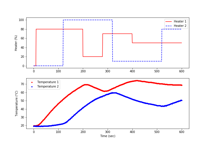
Step Test to Obtain Data
Start the exercise by collecting heater step test data from the device.

import pandas as pd
import tclab
import time
import os.path
# generate step test data on Arduino
filename = 'data.csv'
# redo data collection?
redo = False
# check if file already exists
if os.path.isfile(filename) and (not redo):
print('File: '+filename+' already exists.')
print('Change redo=True to collect data again')
print('TCLab should be at room temperature at start')
else:
# heater steps
Q1d = np.zeros(601)
Q1d[10:200] = 80
Q1d[200:280] = 20
Q1d[280:400] = 70
Q1d[400:] = 50
Q2d = np.zeros(601)
Q2d[120:320] = 100
Q2d[320:520] = 10
Q2d[520:] = 80
# Connect to Arduino
a = tclab.TCLab()
fid = open(filename,'w')
fid.write('Time,Q1,Q2,T1,T2\n')
fid.close()
# run step test (10 min)
for i in range(601):
# set heater values
a.Q1(Q1d[i])
a.Q2(Q2d[i])
print('Time: ' + str(i) + \
' Q1: ' + str(Q1d[i]) + \
' Q2: ' + str(Q2d[i]) + \
' T1: ' + str(a.T1) + \
' T2: ' + str(a.T2))
# wait 1 second
time.sleep(1)
fid = open(filename,'a')
fid.write(str(i)+','+str(Q1d[i])+','+str(Q2d[i])+',' \
+str(a.T1)+','+str(a.T2)+'\n')
# close connection to Arduino
a.close()
fid.close()
Graphical FOPDT Model Fit


import pandas as pd
import matplotlib.pyplot as plt
from scipy.integrate import odeint
import ipywidgets as wg
from IPython.display import display
from IPython.display import clear_output
# try to read local data file first
try:
filename = 'data.csv'
data = pd.read_csv(filename)
except:
filename = 'http://apmonitor.com/pdc/uploads/Main/tclab_data2.txt'
data = pd.read_csv(filename)
n = 601 # time points to plot
tf = 600.0 # final time
# Use expected room temperature for initial condition
#y0 = [23.0,23.0]
# Use initial condition
y0d = [data['T1'].values[0],data['T2'].values[0]]
# load data
Q1 = data['Q1'].values
Q2 = data['Q2'].values
T1 = data['T1'].values
T2 = data['T2'].values
T1p = np.ones(n)*y0d[0]
T2p = np.ones(n)*y0d[1]
def process(y,t,u1,u2,Kp,Kd,taup):
y1,y2 = y
dy1dt = (1.0/taup) * (-(y1-y0d[0]) + Kp * u1 + Kd * (y2-y1))
dy2dt = (1.0/taup) * (-(y2-y0d[1]) + (Kp/2.0) * u2 + Kd * (y1-y2))
return [dy1dt,dy2dt]
def fopdtPlot(Kp,Kd,taup,thetap):
y0 = y0d
t = np.linspace(0,tf,n) # create time vector
iae = 0.0
# loop through all time steps
for i in range(1,n):
# simulate process for one time step
ts = [t[i-1],t[i]] # time interval
inputs = (Q1[max(0,i-int(thetap))],Q2[max(0,i-int(thetap))],Kp,Kd,taup)
y = odeint(process,y0,ts,args=inputs)
y0 = y[1] # record new initial condition
T1p[i] = y0[0]
T2p[i] = y0[1]
iae += np.abs(T1[i]-T1p[i]) + np.abs(T2[i]-T2p[i])
# plot FOPDT response
plt.figure(1,figsize=(15,7))
clear_output()
plt.subplot(2,1,1)
plt.plot(t,T1,'r.',linewidth=2,label='Temperature 1 (meas)')
plt.plot(t,T2,'b.',linewidth=2,label='Temperature 2 (meas)')
plt.plot(t,T1p,'r--',linewidth=2,label='Temperature 1 (pred)')
plt.plot(t,T2p,'b--',linewidth=2,label='Temperature 2 (pred)')
plt.ylabel(r'T $(^oC)$')
plt.text(200,20,'Integral Abs Error: ' + str(np.round(iae,2)))
plt.text(400,35,r'$K_p$: ' + str(np.round(Kp,2)))
plt.text(400,30,r'$K_d$: ' + str(np.round(Kd,2)))
plt.text(400,25,r'$\tau_p$: ' + str(np.round(taup,0)) + ' sec')
plt.text(400,20,r'$\theta_p$: ' + str(np.round(thetap,0)) + ' sec')
plt.legend(loc=2)
plt.subplot(2,1,2)
plt.plot(t,Q1,'b--',linewidth=2,label=r'Heater 1 ($Q_1$)')
plt.plot(t,Q2,'r:',linewidth=2,label=r'Heater 2 ($Q_2$)')
plt.legend(loc='best')
plt.xlabel('time (sec)')
plt.show()
Kp_slide = wg.FloatSlider(value=0.5,min=0.1,max=1.5,step=0.05)
Kd_slide = wg.FloatSlider(value=0.0,min=0.0,max=1.0,step=0.05)
taup_slide = wg.FloatSlider(value=50.0,min=50.0,max=250.0,step=5.0)
thetap_slide = wg.FloatSlider(value=0,min=0,max=30,step=1)
wg.interact(fopdtPlot, Kp=Kp_slide, Kd=Kd_slide, taup=taup_slide,thetap=thetap_slide)
print('FOPDT Simulator: Adjust Kp, Kd, taup, and thetap ' + \
'to achieve lowest Integral Abs Error')
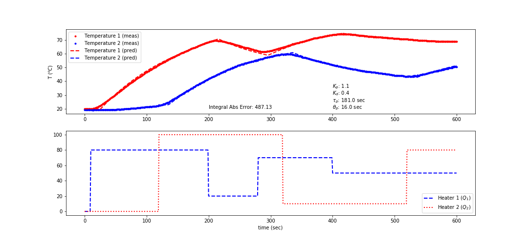
Optimized FOPDT Model Fit
import pandas as pd
import matplotlib.pyplot as plt
%matplotlib inline
from scipy.integrate import odeint
from scipy.optimize import minimize
from scipy.interpolate import interp1d
# initial guesses
x0 = np.zeros(4)
x0[0] = 0.8 # Kp
x0[1] = 0.2 # Kd
x0[2] = 150.0 # taup
x0[3] = 10.0 # thetap
# Import CSV data file
# try to read local data file first
try:
filename = 'data.csv'
data = pd.read_csv(filename)
except:
filename = 'http://apmonitor.com/pdc/uploads/Main/tclab_data2.txt'
data = pd.read_csv(filename)
Q1_0 = data['Q1'].values[0]
Q2_0 = data['Q2'].values[0]
T1_0 = data['T1'].values[0]
T2_0 = data['T2'].values[0]
t = data['Time'].values - data['Time'].values[0]
Q1 = data['Q1'].values
Q2 = data['Q2'].values
T1 = data['T1'].values
T2 = data['T2'].values
# specify number of steps
ns = len(t)
delta_t = t[1]-t[0]
# create linear interpolation of the u data versus time
Qf1 = interp1d(t,Q1)
Qf2 = interp1d(t,Q2)
# define first-order plus dead-time approximation
def fopdt(T,t,Qf1,Qf2,Kp,Kd,taup,thetap):
# T = states
# t = time
# Qf1 = input linear function (for time shift)
# Qf2 = input linear function (for time shift)
# Kp = model gain
# Kd = disturbance gain
# taup = model time constant
# thetap = model time constant
# time-shift Q
try:
if (t-thetap) <= 0:
Qm1 = Qf1(0.0)
Qm2 = Qf2(0.0)
else:
Qm1 = Qf1(t-thetap)
Qm2 = Qf2(t-thetap)
except:
Qm1 = Q1_0
Qm2 = Q2_0
# calculate derivative
dT1dt = (-(T[0]-T1_0) + Kp*(Qm1-Q1_0) + Kd*(T[1]-T[0]))/taup
dT2dt = (-(T[1]-T2_0) + (Kp/2.0)*(Qm2-Q2_0) + Kd*(T[0]-T[1]))/taup
return [dT1dt,dT2dt]
# simulate FOPDT model
def sim_model(x):
# input arguments
Kp,Kd,taup,thetap = x
# storage for model values
T1p = np.ones(ns) * T1_0
T2p = np.ones(ns) * T2_0
# loop through time steps
for i in range(0,ns-1):
ts = [t[i],t[i+1]]
T = odeint(fopdt,[T1p[i],T2p[i]],ts,args=(Qf1,Qf2,Kp,Kd,taup,thetap))
T1p[i+1] = T[-1,0]
T2p[i+1] = T[-1,1]
return T1p,T2p
# define objective
def objective(x):
# simulate model
T1p,T2p = sim_model(x)
# return objective
return sum(np.abs(T1p-T1)+np.abs(T2p-T2))
# show initial objective
print('Initial SSE Objective: ' + str(objective(x0)))
print('Optimizing Values...')
# optimize without parameter constraints
#solution = minimize(objective,x0)
# optimize with bounds on variables
bnds = ((0.4, 1.5), (0.1, 0.5), (50.0, 200.0), (0.0, 30.0))
solution = minimize(objective,x0,bounds=bnds,method='SLSQP')
# show final objective
x = solution.x
iae = objective(x)
Kp,Kd,taup,thetap = x
print('Final SSE Objective: ' + str(objective(x)))
print('Kp: ' + str(Kp))
print('Kd: ' + str(Kd))
print('taup: ' + str(taup))
print('thetap: ' + str(thetap))
# save fopdt.txt file
fid = open('fopdt.txt','w')
fid.write(str(Kp)+'\n')
fid.write(str(Kd)+'\n')
fid.write(str(taup)+'\n')
fid.write(str(thetap)+'\n')
fid.write(str(T1_0)+'\n')
fid.write(str(T2_0)+'\n')
fid.close()
# calculate model with updated parameters
T1p,T2p = sim_model(x)
plt.figure(1,figsize=(15,7))
plt.subplot(2,1,1)
plt.plot(t,T1,'r.',linewidth=2,label='Temperature 1 (meas)')
plt.plot(t,T2,'b.',linewidth=2,label='Temperature 2 (meas)')
plt.plot(t,T1p,'r--',linewidth=2,label='Temperature 1 (pred)')
plt.plot(t,T2p,'b--',linewidth=2,label='Temperature 2 (pred)')
plt.ylabel(r'T $(^oC)$')
plt.text(200,20,'Integral Abs Error: ' + str(np.round(iae,2)))
plt.text(400,35,r'$K_p$: ' + str(np.round(Kp,2)))
plt.text(400,30,r'$K_d$: ' + str(np.round(Kd,2)))
plt.text(400,25,r'$\tau_p$: ' + str(np.round(taup,1)) + ' sec')
plt.text(400,20,r'$\theta_p$: ' + str(np.round(thetap,1)) + ' sec')
plt.legend(loc=2)
plt.subplot(2,1,2)
plt.plot(t,Q1,'b--',linewidth=2,label=r'Heater 1 ($Q_1$)')
plt.plot(t,Q2,'r:',linewidth=2,label=r'Heater 2 ($Q_2$)')
plt.legend(loc='best')
plt.xlabel('time (sec)')
plt.show()
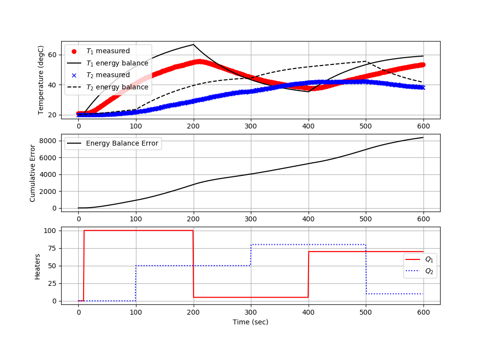
Test Dual Heater Physics-based Model
MATLAB Energy Balance Test
Python Energy Balance Test
import numpy as np
import time
import matplotlib.pyplot as plt
from scipy.integrate import odeint
# define energy balance model
def heat(x,t,Q1,Q2):
# Parameters
Ta = 23 + 273.15 # K
U = 10.0 # W/m^2-K
m = 4.0/1000.0 # kg
Cp = 0.5 * 1000.0 # J/kg-K
A = 10.0 / 100.0**2 # Area in m^2
As = 2.0 / 100.0**2 # Area in m^2
alpha1 = 0.0100 # W / % heater 1
alpha2 = 0.0075 # W / % heater 2
eps = 0.9 # Emissivity
sigma = 5.67e-8 # Stefan-Boltzman
# Temperature States
T1 = x[0]
T2 = x[1]
# Heat Transfer Exchange Between 1 and 2
conv12 = U*As*(T2-T1)
rad12 = eps*sigma*As * (T2**4 - T1**4)
# Nonlinear Energy Balances
dT1dt = (1.0/(m*Cp))*(U*A*(Ta-T1) \
+ eps * sigma * A * (Ta**4 - T1**4) \
+ conv12 + rad12 \
+ alpha1*Q1)
dT2dt = (1.0/(m*Cp))*(U*A*(Ta-T2) \
+ eps * sigma * A * (Ta**4 - T2**4) \
- conv12 - rad12 \
+ alpha2*Q2)
return [dT1dt,dT2dt]
# save txt file
def save_txt(t,u1,u2,y1,y2,sp1,sp2):
data = np.vstack((t,u1,u2,y1,y2,sp1,sp2)) # vertical stack
data = data.T # transpose data
top = 'Time (sec), Heater 1 (%), Heater 2 (%), ' \
+ 'Temperature 1 (degC), Temperature 2 (degC), ' \
+ 'Set Point 1 (degC), Set Point 2 (degC)'
np.savetxt('data.txt',data,delimiter=',',header=top,comments='')
# Connect to Arduino
a = tclab.TCLab()
# Turn LED on
print('LED On')
a.LED(100)
# Run time in minutes
run_time = 10.0
# Number of cycles
loops = int(60.0*run_time)
tm = np.zeros(loops)
# Temperature (K)
Tsp1 = np.ones(loops) * 23.0 # set point (degC)
T1 = np.ones(loops) * a.T1 # measured T (degC)
Tsp2 = np.ones(loops) * 23.0 # set point (degC)
T2 = np.ones(loops) * a.T2 # measured T (degC)
# Predictions
Tp1 = np.ones(loops) * a.T1
Tp2 = np.ones(loops) * a.T2
error_eb = np.zeros(loops)
# impulse tests (0 - 100%)
Q1 = np.ones(loops) * 0.0
Q2 = np.ones(loops) * 0.0
# steps
Q1[10:] = 100.0
Q2[100:] = 50.0
Q1[200:] = 5.0
Q2[300:] = 80.0
Q1[400:] = 70.0
Q2[500:] = 10.0
print('Running Main Loop. Ctrl-C to end.')
print(' Time Q1 Q2 T1 T2')
print('{:6.1f} {:6.2f} {:6.2f} {:6.2f} {:6.2f}'.format(tm[0], \
Q1[0], \
Q2[0], \
T1[0], \
T2[0]))
# Create plot
plt.figure(figsize=(10,7))
plt.ion()
plt.show()
# Main Loop
start_time = time.time()
prev_time = start_time
try:
for i in range(1,loops):
# Sleep time
sleep_max = 1.0
sleep = sleep_max - (time.time() - prev_time)
if sleep>=0.01:
time.sleep(sleep-0.01)
else:
time.sleep(0.01)
# Record time and change in time
t = time.time()
dt = t - prev_time
prev_time = t
tm[i] = t - start_time
# Read temperatures in Kelvin
T1[i] = a.T1
T2[i] = a.T2
# Simulate one time step with Energy Balance
Tinit = [Tp1[i-1]+273.15,Tp2[i-1]+273.15]
Tnext = odeint(heat,Tinit, \
[0,dt],args=(Q1[i-1],Q2[i-1]))
Tp1[i] = Tnext[1,0]-273.15
Tp2[i] = Tnext[1,1]-273.15
error_eb[i] = error_eb[i-1] \
+ (abs(Tp1[i]-T1[i]) \
+ abs(Tp2[i]-T2[i]))*dt
# Write output (0-100)
a.Q1(Q1[i])
a.Q2(Q2[i])
# Print line of data
print('{:6.1f} {:6.2f} {:6.2f} {:6.2f} {:6.2f}'.format(tm[i], \
Q1[i], \
Q2[i], \
T1[i], \
T2[i]))
# Plot
plt.clf()
ax=plt.subplot(3,1,1)
ax.grid()
plt.plot(tm[0:i],T1[0:i],'ro',label=r'$T_1$ measured')
plt.plot(tm[0:i],Tp1[0:i],'k-',label=r'$T_1$ energy balance')
plt.plot(tm[0:i],T2[0:i],'bx',label=r'$T_2$ measured')
plt.plot(tm[0:i],Tp2[0:i],'k--',label=r'$T_2$ energy balance')
plt.ylabel('Temperature (degC)')
plt.legend(loc=2)
ax=plt.subplot(3,1,2)
ax.grid()
plt.plot(tm[0:i],error_eb[0:i],'k-',label='Energy Balance Error')
plt.ylabel('Cumulative Error')
plt.legend(loc='best')
ax=plt.subplot(3,1,3)
ax.grid()
plt.plot(tm[0:i],Q1[0:i],'r-',label=r'$Q_1$')
plt.plot(tm[0:i],Q2[0:i],'b:',label=r'$Q_2$')
plt.ylabel('Heaters')
plt.xlabel('Time (sec)')
plt.legend(loc='best')
plt.draw()
plt.pause(0.05)
# Turn off heaters
a.Q1(0)
a.Q2(0)
# Save text file and plot at end
save_txt(tm[0:i],Q1[0:i],Q2[0:i],T1[0:i],T2[0:i],Tsp1[0:i],Tsp2[0:i])
# Save figure
plt.savefig('test_Models.png')
# Allow user to end loop with Ctrl-C
except KeyboardInterrupt:
# Disconnect from Arduino
a.Q1(0)
a.Q2(0)
print('Shutting down')
a.close()
save_txt(tm[0:i],Q1[0:i],Q2[0:i],T1[0:i],T2[0:i],Tsp1[0:i],Tsp2[0:i])
plt.savefig('test_Models.png')
# Make sure serial connection still closes when there's an error
except:
# Disconnect from Arduino
a.Q1(0)
a.Q2(0)
print('Error: Shutting down')
a.close()
save_txt(tm[0:i],Q1[0:i],Q2[0:i],T1[0:i],T2[0:i],Tsp1[0:i],Tsp2[0:i])
plt.savefig('test_Models.png')
raise
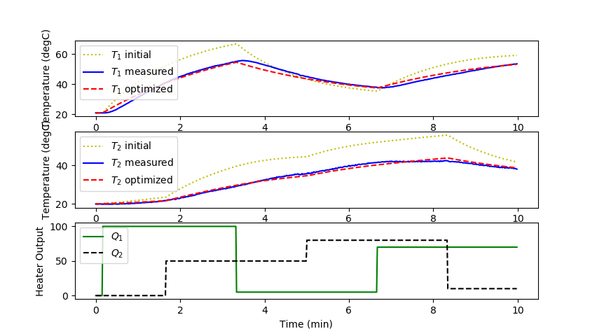
Fit First-Order Physics-based Model with Optimization
Starting with the dual heater energy balances, adjust parameters such as `U` the heat transfer coefficient, `\alpha_1` or `\alpha_2` the heater power factors, or other uncertain parameters that will improve the fit to the data. Other factors such as the ambient temperature (`T_\infty`), can be updated by noting the temperature when the device is cool and the heaters are initially off.
Parameter Estimation with Python Scipy
import matplotlib.pyplot as plt
from scipy.integrate import odeint
from scipy.optimize import minimize
import pandas as pd
# generate data file from TCLab or get sample data file from:
# https://apmonitor.com/pdc/index.php/Main/ArduinoEstimation2
# Import data file
# Column 1 = time (t)
# Column 2 = input (u)
# Column 3 = output (yp)
data = np.loadtxt('data.txt',delimiter=',',skiprows=1)
# extract data columns
t = data[:,0].T
Q1 = data[:,1].T
Q2 = data[:,2].T
T1meas = data[:,3].T
T2meas = data[:,4].T
# number of time points
ns = len(t)
# define energy balance model
def heat(x,t,Q1,Q2,p):
# Optimized parameters
U,alpha1,alpha2 = p
# Parameters
Ta = 23 + 273.15 # K
m = 4.0/1000.0 # kg
Cp = 0.5 * 1000.0 # J/kg-K
A = 10.0 / 100.0**2 # Area in m^2
As = 2.0 / 100.0**2 # Area in m^2
eps = 0.9 # Emissivity
sigma = 5.67e-8 # Stefan-Boltzman
# Temperature States
T1 = x[0] + 273.15
T2 = x[1] + 273.15
# Heat Transfer Exchange Between 1 and 2
conv12 = U*As*(T2-T1)
rad12 = eps*sigma*As * (T2**4 - T1**4)
# Nonlinear Energy Balances
dT1dt = (1.0/(m*Cp))*(U*A*(Ta-T1) \
+ eps * sigma * A * (Ta**4 - T1**4) \
+ conv12 + rad12 \
+ alpha1*Q1)
dT2dt = (1.0/(m*Cp))*(U*A*(Ta-T2) \
+ eps * sigma * A * (Ta**4 - T2**4) \
- conv12 - rad12 \
+ alpha2*Q2)
return [dT1dt,dT2dt]
def simulate(p):
T = np.zeros((len(t),2))
T[0,0] = T1meas[0]
T[0,1] = T2meas[0]
T0 = T[0]
for i in range(len(t)-1):
ts = [t[i],t[i+1]]
y = odeint(heat,T0,ts,args=(Q1[i],Q2[i],p))
T0 = y[-1]
T[i+1] = T0
return T
# define objective
def objective(p):
# simulate model
Tp = simulate(p)
# calculate objective
obj = 0.0
for i in range(len(t)):
obj += ((Tp[i,0]-T1meas[i])/T1meas[i])**2 \
+((Tp[i,1]-T2meas[i])/T2meas[i])**2
# return result
return obj
# Parameter initial guess
U = 10.0 # Heat transfer coefficient (W/m^2-K)
alpha1 = 0.0100 # Heat gain 1 (W/%)
alpha2 = 0.0075 # Heat gain 2 (W/%)
p0 = [U,alpha1,alpha2]
# show initial objective
print('Initial SSE Objective: ' + str(objective(p0)))
# optimize parameters
# bounds on variables
bnds = ((2.0, 20.0),(0.005,0.02),(0.002,0.015))
solution = minimize(objective,p0,method='SLSQP',bounds=bnds)
p = solution.x
# show final objective
print('Final SSE Objective: ' + str(objective(p)))
# optimized parameter values
U = p[0]
alpha1 = p[1]
alpha2 = p[2]
print('U: ' + str(U))
print('alpha1: ' + str(alpha1))
print('alpha2: ' + str(alpha2))
# calculate model with updated parameters
Ti = simulate(p0)
Tp = simulate(p)
# Plot results
plt.figure(1)
plt.subplot(3,1,1)
plt.plot(t/60.0,Ti[:,0],'y:',label=r'$T_1$ initial')
plt.plot(t/60.0,T1meas,'b-',label=r'$T_1$ measured')
plt.plot(t/60.0,Tp[:,0],'r--',label=r'$T_1$ optimized')
plt.ylabel('Temperature (degC)')
plt.legend(loc='best')
plt.subplot(3,1,2)
plt.plot(t/60.0,Ti[:,1],'y:',label=r'$T_2$ initial')
plt.plot(t/60.0,T2meas,'b-',label=r'$T_2$ measured')
plt.plot(t/60.0,Tp[:,1],'r--',label=r'$T_2$ optimized')
plt.ylabel('Temperature (degC)')
plt.legend(loc='best')
plt.subplot(3,1,3)
plt.plot(t/60.0,Q1,'g-',label=r'$Q_1$')
plt.plot(t/60.0,Q2,'k--',label=r'$Q_2$')
plt.ylabel('Heater Output')
plt.legend(loc='best')
plt.xlabel('Time (min)')
plt.show()
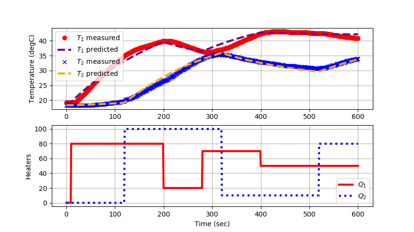
Parameter Estimation with Python GEKKO
import matplotlib.pyplot as plt
import pandas as pd
from gekko import GEKKO
# Import or generate data
filename = 'tclab_dyn_data2.csv'
try:
data = pd.read_csv(filename)
except:
url = 'http://apmonitor.com/do/uploads/Main/tclab_dyn_data2.txt'
data = pd.read_csv(url)
# Create GEKKO Model
m = GEKKO()
m.time = data['Time'].values
# Parameters to Estimate
U = m.FV(value=10,lb=1,ub=20)
alpha1 = m.FV(value=0.01,lb=0.003,ub=0.03) # W / % heater
alpha2 = m.FV(value=0.005,lb=0.002,ub=0.02) # W / % heater
# STATUS=1 allows solver to adjust parameter
U.STATUS = 1
alpha1.STATUS = 1
alpha2.STATUS = 1
# Measured inputs
Q1 = m.MV(value=data['H1'].values)
Q2 = m.MV(value=data['H2'].values)
# State variables
TC1 = m.CV(value=data['T1'].values)
TC1.FSTATUS = 1 # minimize fstatus * (meas-pred)^2
TC2 = m.CV(value=data['T2'].values)
TC2.FSTATUS = 1 # minimize fstatus * (meas-pred)^2
Ta = m.Param(value=19.0+273.15) # K
mass = m.Param(value=4.0/1000.0) # kg
Cp = m.Param(value=0.5*1000.0) # J/kg-K
A = m.Param(value=10.0/100.0**2) # Area not between heaters in m^2
As = m.Param(value=2.0/100.0**2) # Area between heaters in m^2
eps = m.Param(value=0.9) # Emissivity
sigma = m.Const(5.67e-8) # Stefan-Boltzmann
# Heater temperatures in Kelvin
T1 = m.Intermediate(TC1+273.15)
T2 = m.Intermediate(TC2+273.15)
# Heat transfer between two heaters
Q_C12 = m.Intermediate(U*As*(T2-T1)) # Convective
Q_R12 = m.Intermediate(eps*sigma*As*(T2**4-T1**4)) # Radiative
# Semi-fundamental correlations (energy balances)
m.Equation(TC1.dt() == (1.0/(mass*Cp))*(U*A*(Ta-T1) \
+ eps * sigma * A * (Ta**4 - T1**4) \
+ Q_C12 + Q_R12 \
+ alpha1*Q1))
m.Equation(TC2.dt() == (1.0/(mass*Cp))*(U*A*(Ta-T2) \
+ eps * sigma * A * (Ta**4 - T2**4) \
- Q_C12 - Q_R12 \
+ alpha2*Q2))
# Options
m.options.IMODE = 5 # MHE
m.options.EV_TYPE = 2 # Objective type
m.options.NODES = 2 # Collocation nodes
m.options.SOLVER = 3 # IPOPT
# Solve
m.solve(disp=True)
# Parameter values
print('U : ' + str(U.value[0]))
print('alpha1: ' + str(alpha1.value[0]))
print('alpha2: ' + str(alpha2.value[0]))
# Create plot
plt.figure()
ax=plt.subplot(2,1,1)
ax.grid()
plt.plot(data['Time'],data['T1'],'ro',label=r'$T_1$ measured')
plt.plot(m.time,TC1.value,color='purple',linestyle='--',\
linewidth=3,label=r'$T_1$ predicted')
plt.plot(data['Time'],data['T2'],'bx',label=r'$T_2$ measured')
plt.plot(m.time,TC2.value,color='orange',linestyle='--',\
linewidth=3,label=r'$T_2$ predicted')
plt.ylabel('Temperature (degC)')
plt.legend(loc=2)
ax=plt.subplot(2,1,2)
ax.grid()
plt.plot(data['Time'],data['H1'],'r-',\
linewidth=3,label=r'$Q_1$')
plt.plot(data['Time'],data['H2'],'b:',\
linewidth=3,label=r'$Q_2$')
plt.ylabel('Heaters')
plt.xlabel('Time (sec)')
plt.legend(loc='best')
plt.show()
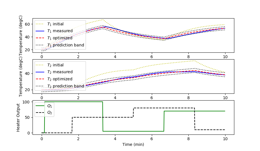
Parameter Estimation with Confidence Intervals
See Regression Statistics Introduction for information on obtaining parameter confidence intervals and data prediction bands.
from scipy.optimize import curve_fit
import uncertainties as unc
import matplotlib.pyplot as plt
import uncertainties.unumpy as unp
from scipy.integrate import odeint
import pandas as pd
from scipy import stats
# calculate lower and upper prediction bands
def predband(x, xd, yd, f_vars, conf=0.95):
"""
Code adapted from Rodrigo Nemmen's post:
https://astropython.blogspot.com.ar/2011/12/calculating-prediction-band-
of-linear.html
Calculates the prediction band of the regression model at the
desired confidence level.
Clarification of the difference between confidence and prediction bands:
"The prediction bands are further from the best-fit line than the
confidence bands, a lot further if you have many data points. The 95%
prediction band is the area in which you expect 95% of all data points
to fall. In contrast, the 95% confidence band is the area that has a
95% chance of containing the true regression line."
(from https://www.graphpad.com/guides/prism/6/curve-fitting/index.htm?
reg_graphing_tips_linear_regressio.htm)
Arguments:
- x: array with x values to calculate the confidence band.
- xd, yd: data arrays.
- a, b, c: linear fit parameters.
- conf: desired confidence level, by default 0.95 (2 sigma)
References:
1. https://www.JerryDallal.com/LHSP/slr.htm, Introduction to Simple Linear
Regression, Gerard E. Dallal, Ph.D.
"""
alpha = 1. - conf # Significance
N = xd.size # data sample size
var_n = len(f_vars) # Number of variables used by the fitted function.
# Quantile of Student's t distribution for p=(1 - alpha/2)
q = stats.t.ppf(1. - alpha / 2., N - var_n)
# Std. deviation of an individual measurement (Bevington, eq. 6.15)
se = np.sqrt(1. / (N - var_n) * np.sum((yd - simulate(xd, *f_vars)) ** 2))
# Auxiliary definitions
sx = (x - xd.mean()) ** 2
sxd = np.sum((xd - xd.mean()) ** 2)
# Predicted values (best-fit model)
yp = simulate(x, *f_vars)
# Prediction band
dy = q * se * np.sqrt(1. + (1. / N) + (sx / sxd))
# Upper & lower prediction bands.
lpb, upb = yp - dy, yp + dy
return lpb, upb
# generate data file from TCLab or get sample data file from:
# https://apmonitor.com/pdc/index.php/Main/ArduinoEstimation2
# Import data file
# Column 1 = time (t)
# Column 2 = input (u)
# Column 3 = output (yp)
data = np.loadtxt('data.txt',delimiter=',',skiprows=1)
# extract data columns
t = data[:,0].T
Q1 = data[:,1].T
Q2 = data[:,2].T
T1meas = data[:,3].T
T2meas = data[:,4].T
ind = np.linspace(0,np.size(t),np.size(t))
# number of time points
ns = len(t)
# define energy balance model
def heat(x,t,Q1,Q2,p):
# Optimized parameters
U,alpha1,alpha2 = p
# Parameters
Ta = 23 + 273.15 # K
m = 4.0/1000.0 # kg
Cp = 0.5 * 1000.0 # J/kg-K
A = 10.0 / 100.0**2 # Area in m^2
As = 2.0 / 100.0**2 # Area in m^2
eps = 0.9 # Emissivity
sigma = 5.67e-8 # Stefan-Boltzman
# Temperature States
T1 = x[0] + 273.15
T2 = x[1] + 273.15
# Heat Transfer Exchange Between 1 and 2
conv12 = U*As*(T2-T1)
rad12 = eps*sigma*As * (T2**4 - T1**4)
# Nonlinear Energy Balances
dT1dt = (1.0/(m*Cp))*(U*A*(Ta-T1) \
+ eps * sigma * A * (Ta**4 - T1**4) \
+ conv12 + rad12 \
+ alpha1*Q1)
dT2dt = (1.0/(m*Cp))*(U*A*(Ta-T2) \
+ eps * sigma * A * (Ta**4 - T2**4) \
- conv12 - rad12 \
+ alpha2*Q2)
return [dT1dt,dT2dt]
def simulate(tm,U,alpha1,alpha2):
T = np.zeros((len(t),2))
T[0,0] = T1meas[0]
T[0,1] = T2meas[0]
T0 = T[0]
p = (U,alpha1,alpha2)
for i in range(len(t)-1):
ts = [t[i],t[i+1]]
y = odeint(heat,T0,ts,args=(Q1[i],Q2[i],p))
T0 = y[-1]
T[i+1] = T0
z = np.empty((len(t)*2))
z[0:len(t)] = T[:,0]
z[len(t):] = T[:,1]
return z
def simulate2(p):
T = np.zeros((len(t),2))
T[0,0] = T1meas[0]
T[0,1] = T2meas[0]
T0 = T[0]
for i in range(len(t)-1):
ts = [t[i],t[i+1]]
y = odeint(heat,T0,ts,args=(Q1[i],Q2[i],p))
T0 = y[-1]
T[i+1] = T0
return T
# Parameter initial guess
U = 10.0 # Heat transfer coefficient (W/m^2-K)
alpha1 = 0.0100 # Heat gain 1 (W/%)
alpha2 = 0.0075 # Heat gain 2 (W/%)
pinit = [U,alpha1,alpha2]
x = []
y = np.empty((len(t)*2))
y[0:len(t)] = T1meas
y[len(t):] = T2meas
popt, pcov = curve_fit(simulate, x, y)
Uu, alpha1u, alpha2u = unc.correlated_values(popt, pcov)
# create prediction band
lpb, upb = predband(y, y, y, popt, conf=0.95)
lpb1 = np.empty((len(t)))
lpb2 = np.empty((len(t)))
upb1 = np.empty((len(t)))
upb2 = np.empty((len(t)))
lpb1[0:len(t)] = lpb[0:len(t)]
lpb2[0:len(t)] = lpb[len(t):]
upb1[0:len(t)] = upb[0:len(t)]
upb2[0:len(t)] = upb[len(t):]
# optimized parameter values with uncertainties
print('Optimal Parameters with Uncertanty Range')
print('U: ' + str(Uu))
print('alpha1: ' + str(alpha1u))
print('alpha2: ' + str(alpha2u))
# calculate model with updated parameters
Ti = simulate2(pinit)
Tp = simulate2(popt)
# Plot results
plt.figure(1)
plt.subplot(3,1,1)
plt.plot(t/60.0,Ti[:,0],'y:',label=r'$T_1$ initial')
plt.plot(t/60.0,T1meas,'b-',label=r'$T_1$ measured')
plt.plot(t/60.0,Tp[:,0],'r--',label=r'$T_1$ optimized')
plt.plot(t/60.0,lpb1,'k:',label=r'$T_1$ prediction band')
plt.plot(t/60.0,upb1,'k:')
plt.ylabel('Temperature (degC)')
plt.legend(loc='best')
plt.subplot(3,1,2)
plt.plot(t/60.0,Ti[:,1],'y:',label=r'$T_2$ initial')
plt.plot(t/60.0,T2meas,'b-',label=r'$T_2$ measured')
plt.plot(t/60.0,Tp[:,1],'r--',label=r'$T_2$ optimized')
plt.plot(t/60.0,lpb2,'k:',label=r'$T_2$ prediction band')
plt.plot(t/60.0,upb2,'k:')
plt.ylabel('Temperature (degC)')
plt.legend(loc='best')
plt.subplot(3,1,3)
plt.plot(t/60.0,Q1,'g-',label=r'$Q_1$')
plt.plot(t/60.0,Q2,'k--',label=r'$Q_2$')
plt.ylabel('Heater Output')
plt.legend(loc='best')
plt.xlabel('Time (min)')
plt.show()
global t T1meas T2meas Q1 Q2
% generate data file from TCLab or get sample data file from:
% https://apmonitor.com/pdc/index.php/Main/ArduinoEstimation2
% Import data file
% Column 1 = time (t)
% Column 2 = input (u)
% Column 3 = output (yp)
filename = 'data.txt';
delimiterIn = ',';
headerlinesIn = 1;
z = importdata(filename,delimiterIn,headerlinesIn);
% extract data columns
t = z.data(:,1);
Q1 = z.data(:,2);
Q2 = z.data(:,3);
T1meas = z.data(:,4);
T2meas = z.data(:,5);
% number of time points
ns = length(t);
% Parameter initial guess
U = 10.0; % Heat transfer coefficient (W/m^2-K)
alpha1 = 0.0100; % Heat gain 1 (W/%)
alpha2 = 0.0075; % Heat gain 2 (W/%)
p0 = [U,alpha1,alpha2];
% show initial objective
disp(['Initial SSE Objective: ' num2str(objective(p0))])
% optimize parameters
% no linear constraints
A = [];
b = [];
Aeq = [];
beq = [];
nlcon = [];
% optimize with fmincon
lb = [2,0.005,0.002]; % lower bound
ub = [20,0.02,0.015]; % upper bound
% options = optimoptions(@fmincon,'Algorithm','interior-point');
p = fmincon(@objective,p0,A,b,Aeq,beq,lb,ub,nlcon); %,options);
% show final objective
disp(['Final SSE Objective: ' num2str(objective(p))])
% optimized parameter values
U = p(1);
alpha1 = p(2);
alpha2 = p(3);
disp(['U: ' num2str(U)])
disp(['alpha1: ' num2str(alpha1)])
disp(['alpha2: ' num2str(alpha2)])
% calculate model with updated parameters
Ti = simulate(p0);
Tp = simulate(p);
% Plot results
figure(1)
subplot(3,1,1)
plot(t/60.0,Ti(:,1),'y:','LineWidth',2)
hold on
plot(t/60.0,T1meas,'b-','LineWidth',2)
plot(t/60.0,Tp(:,1),'r--','LineWidth',2)
ylabel('Temperature (degC)')
legend('T_1 initial','T_1 measured','T_1 optimized')
subplot(3,1,2)
plot(t/60.0,Ti(:,2),'y:','LineWidth',2)
hold on
plot(t/60.0,T2meas,'b-','LineWidth',2)
plot(t/60.0,Tp(:,2),'r--','LineWidth',2)
ylabel('Temperature (degC)')
legend('T_2 initial','T_2 measured','T_2 optimized')
subplot(3,1,3)
plot(t/60.0,Q1,'g-','LineWidth',2)
hold on
plot(t/60.0,Q2,'k--','LineWidth',2)
ylabel('Heater Output')
legend('Q_1','Q_2')
xlabel('Time (min)')
Save as heat.m
function dTdt = heat(t,x,Q1,Q2,p)
%U = 10.0; % W/m^2-K
%alpha1 = 0.0100; % W / % heater 1
%alpha2 = 0.0075; % W / % heater 2
U = p(1);
alpha1 = p(2);
alpha2 = p(3);
% Parameters
Ta = 23 + 273.15; % K
m = 4.0/1000.0; % kg
Cp = 0.5 * 1000.0; % J/kg-K
A = 10.0 / 100.0^2; % Area in m^2
As = 2.0 / 100.0^2; % Area in m^2
eps = 0.9; % Emissivity
sigma = 5.67e-8; % Stefan-Boltzman
% Temperature States
T1 = x(1)+273.15;
T2 = x(2)+273.15;
% Heat Transfer Exchange Between 1 and 2
conv12 = U*As*(T2-T1);
rad12 = eps*sigma*As * (T2^4 - T1^4);
% Nonlinear Energy Balances
dT1dt = (1.0/(m*Cp))*(U*A*(Ta-T1) ...
+ eps * sigma * A * (Ta^4 - T1^4) ...
+ conv12 + rad12 ...
+ alpha1*Q1);
dT2dt = (1.0/(m*Cp))*(U*A*(Ta-T2) ...
+ eps * sigma * A * (Ta^4 - T2^4) ...
- conv12 - rad12 ...
+ alpha2*Q2);
dTdt = [dT1dt,dT2dt]';
end
Save as simulate.m
global t T1meas T2meas Q1 Q2
T = zeros(length(t),2);
T(1,1) = T1meas(1);
T(1,2) = T2meas(1);
T0 = [T(1,1),T(1,2)];
for i = 1:length(t)-1
ts = [t(i),t(i+1)];
sol = ode15s(@(t,x)heat(t,x,Q1(i),Q2(i),p),ts,T0);
T0 = [sol.y(1,end),sol.y(2,end)];
T(i+1,1) = T0(1);
T(i+1,2) = T0(2);
end
end
Save as objective.m
function obj = objective(p)
global T1meas T2meas
% simulate model
Tp = simulate(p);
% calculate objective
obj = sum(((Tp(:,1)-T1meas)./T1meas).^2) ...
+ sum(((Tp(:,2)-T2meas)./T2meas).^2);
end
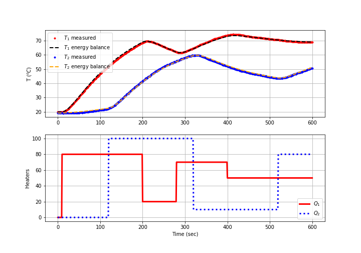
Fit Second-Order Physics-based Model with Optimization
A second-order physics-based model starts with the dual heater energy balances but adds additional equations for the conduction of heat from the heater to the temperature sensor. The heat loss by convection and conduction from the thermistor sensor is assumed to be negligible and the principal heat transfer is by conduction. The temperatures of the heaters `T_{H1}` and `T_{H1}` are related to the temperatures of the sensors `T_{C1}` and `T_{C1}` with a discretized version of Fourier's law with thermal conductivity (k), cross-section area for conduction (A), and distance between the heater and sensor `\Delta x`.
$$m \, c_p \, \frac{dT_{C1}}{dt} = \frac{k\,A_c}{\Delta x} \left( T_{H1} - T_{C1} \right)$$
$$m \, c_p \, \frac{dT_{C2}}{dt} = \frac{k\,A_c}{\Delta x} \left( T_{H2} - T_{C2} \right)$$
The time constant form of the conduction equation is obtained by defining `\tau` for all the parameters that are lumped into a single constant.
$$\tau = \frac{m \, c_p \, \Delta x}{k\,A_c}$$
The new equation is a standard first order linear system that relates the heater actuator temperature to the sensor where the temperature is physically measured.
$$\tau \frac{dT_{C1}}{dt} = T_{H1} - T_{C1}$$
$$\tau \frac{dT_{C2}}{dt} = T_{H2} - T_{C2}$$
In this regression, parameters `U`, `U_s`, `\alpha_1`, `\alpha_2`, and `\tau` are adjusted to minimize the model error objective function. The additional `U_s` is the modified heat transfer coefficient between the heaters that is higher than the heat transfer coefficient from natural convection.
Parameter Regression (2nd Order) with Python GEKKO
import matplotlib.pyplot as plt
import pandas as pd
from gekko import GEKKO
from scipy.integrate import odeint
from scipy.interpolate import interp1d
# Import data
try:
# try to read local data file first
filename = 'data.csv'
data = pd.read_csv(filename)
except:
filename = 'https://apmonitor.com/pdc/uploads/Main/tclab_data2.txt'
data = pd.read_csv(filename)
# Fit Parameters of Energy Balance
m = GEKKO() # Create GEKKO Model
# Parameters to Estimate
U = m.FV(value=10,lb=1,ub=20)
Us = m.FV(value=20,lb=5,ub=40)
alpha1 = m.FV(value=0.01,lb=0.001,ub=0.03) # W / % heater
alpha2 = m.FV(value=0.005,lb=0.001,ub=0.02) # W / % heater
tau = m.FV(value=10.0,lb=5.0,ub=60.0)
# Measured inputs
Q1 = m.Param()
Q2 = m.Param()
Ta =23.0+273.15 # K
mass = 4.0/1000.0 # kg
Cp = 0.5*1000.0 # J/kg-K
A = 10.0/100.0**2 # Area not between heaters in m^2
As = 2.0/100.0**2 # Area between heaters in m^2
eps = 0.9 # Emissivity
sigma = 5.67e-8 # Stefan-Boltzmann
TH1 = m.SV()
TH2 = m.SV()
TC1 = m.CV()
TC2 = m.CV()
# Heater Temperatures in Kelvin
T1 = m.Intermediate(TH1+273.15)
T2 = m.Intermediate(TH2+273.15)
# Heat transfer between two heaters
Q_C12 = m.Intermediate(Us*As*(T2-T1)) # Convective
Q_R12 = m.Intermediate(eps*sigma*As*(T2**4-T1**4)) # Radiative
# Energy balances
m.Equation(TH1.dt() == (1.0/(mass*Cp))*(U*A*(Ta-T1) \
+ eps * sigma * A * (Ta**4 - T1**4) \
+ Q_C12 + Q_R12 \
+ alpha1*Q1))
m.Equation(TH2.dt() == (1.0/(mass*Cp))*(U*A*(Ta-T2) \
+ eps * sigma * A * (Ta**4 - T2**4) \
- Q_C12 - Q_R12 \
+ alpha2*Q2))
# Conduction to temperature sensors
m.Equation(tau*TC1.dt() == TH1-TC1)
m.Equation(tau*TC2.dt() == TH2-TC2)
# Options
# STATUS=1 allows solver to adjust parameter
U.STATUS = 1
Us.STATUS = 1
alpha1.STATUS = 1
alpha2.STATUS = 1
tau.STATUS = 1
Q1.value=data['Q1'].values
Q2.value=data['Q2'].values
TH1.value=data['T1'].values[0]
TH2.value=data['T2'].values[0]
TC1.value=data['T1'].values
TC1.FSTATUS = 1 # minimize fstatus * (meas-pred)^2
TC2.value=data['T2'].values
TC2.FSTATUS = 1 # minimize fstatus * (meas-pred)^2
m.time = data['Time'].values
m.options.IMODE = 5 # MHE
m.options.EV_TYPE = 2 # Objective type
m.options.NODES = 2 # Collocation nodes
m.options.SOLVER = 3 # IPOPT
m.solve(disp=False) # Solve
# Parameter values
print('U : ' + str(U.value[0]))
print('Us : ' + str(Us.value[0]))
print('alpha1: ' + str(alpha1.value[0]))
print('alpha2: ' + str(alpha2.value[-1]))
print('tau: ' + str(tau.value[0]))
sae = 0.0
for i in range(len(data)):
sae += np.abs(data['T1'][i]-TC1.value[i])
sae += np.abs(data['T2'][i]-TC2.value[i])
print('SAE Energy Balance: ' + str(sae))
# Create plot
plt.figure(figsize=(10,7))
ax=plt.subplot(2,1,1)
ax.grid()
plt.plot(data['Time'],data['T1'],'r.',label=r'$T_1$ measured')
plt.plot(m.time,TC1.value,color='black',linestyle='--',\
linewidth=2,label=r'$T_1$ energy balance')
plt.plot(data['Time'],data['T2'],'b.',label=r'$T_2$ measured')
plt.plot(m.time,TC2.value,color='orange',linestyle='--',\
linewidth=2,label=r'$T_2$ energy balance')
plt.ylabel(r'T ($^oC$)')
plt.legend(loc=2)
ax=plt.subplot(2,1,2)
ax.grid()
plt.plot(data['Time'],data['Q1'],'r-',\
linewidth=3,label=r'$Q_1$')
plt.plot(data['Time'],data['Q2'],'b:',\
linewidth=3,label=r'$Q_2$')
plt.ylabel('Heaters')
plt.xlabel('Time (sec)')
plt.legend(loc='best')
plt.savefig('tclab_2nd_order_physics.png')
plt.show()
Return to Temperature Control Lab Overview