Arduino Dynamic Temperature Modeling
Objective: Derive a nonlinear transient model and fit a linear first order or second order system. Compare the model predictions to the transient lab data.
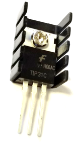
The first phase of the temperature control lab is to derive a dynamic model of the system with guess values for parameters. The three important elements for a control loop are the measurement device (thermistor temperature sensor), an actuator (transistor), and capability to perform computerized control (USB interface). At maximum output the transistor dissipates 1 W of power at 100% heater output. The mass of the transistor and heat sink with fins is 4 gm.
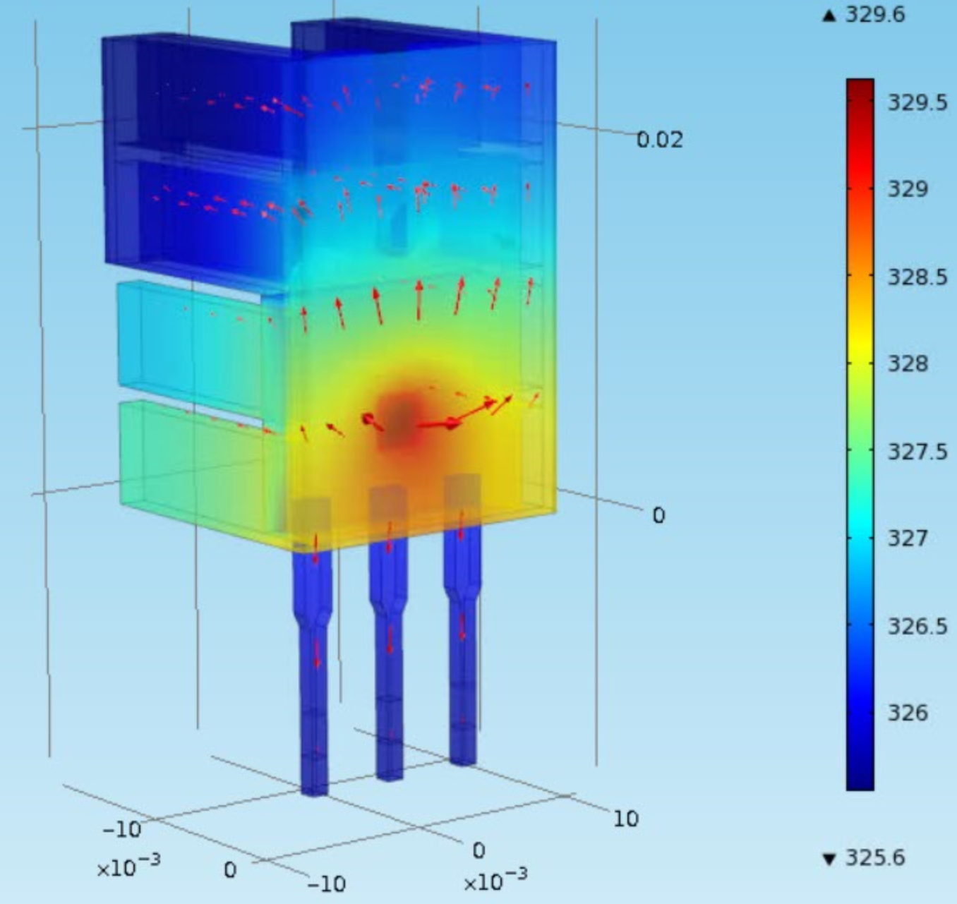
Steel has a heat capacity of 500 `J/{kg K}`. The surface area of the heater and sensor is about 12 `cm^2`. A convective heat transfer coefficient for quiescent air is approximately 10 `W/{m^2K}`. The heat generated by the transistor transfers away from the device primarily by convection but radiative heat transfer may also be a contributing factor. The radiative heat transfer can be included in the model to determine what fraction of heat is lost by convection and heat radiation. Heat transfer is improved with a thermal coupling (white epoxy) that connects the two components.
| Quantity | Value |
| Initial temperature (T0) | 296.15 K (23oC) |
| Ambient temperature (`T_\infty`) | 296.15 K (23oC) |
| Heater output (Q) | 0 to 1 W |
| Heater factor (`\alpha`) | 0.01 W/(% heater) |
| Heat capacity (Cp) | 500 J/kg-K |
| Surface Area (A) | 1.2x10⁻³ m2 (12 cm2) |
| Mass (m) | 0.004 kg (4 gm) |
| Overall Heat Transfer Coefficient (U) | 10 W/m2-K |
| Emissivity (`\epsilon`) | 0.9 |
| Stefan Boltzmann Constant (`\sigma`) | 5.67x10⁻⁸ W/m2-K4 |
Create a dynamic model of the dynamic response between input power to the transistor and the temperature sensed by the thermistor. Use an energy balance to start the derivation.
$$m\,c_p\frac{dT}{dt} = \sum \dot h_{in} - \sum \dot h_{out} + Q$$
Expand or simplify terms that are needed for this application. The full energy balance includes convection and radiation terms.
$$m\,c_p\frac{dT}{dt} = U\,A\,\left(T_\infty-T\right) + \epsilon\,\sigma\,A\,\left(T_\infty^4-T^4\right) + \alpha Q$$
where `m` is the mass, `c_p` is the heat capacity, `T` is the temperature, `U` is the heat transfer coefficient, `A` is the area, `T_\infty` is the ambient temperature, `\epsilon=0.9` is the emissivity, `\sigma =` 5.67x10⁻⁸ `W/{m^2 K^4}` is the Stefan-Boltzmann constant, and `Q` is the percentage heater output. The parameter `\alpha` is a factor that relates heater output (0-100%) to power dissipated by the transistor in Watts. Use this equation to develop a dynamic simulation of the temperature response due to an impulse (off, on, off) in the heater output. Leave the heater on for sufficient time to observe nearly steady state conditions.
Single Heater Model
import matplotlib.pyplot as plt
from scipy.integrate import odeint
# define energy balance model
def heat(x,t,Q):
# Parameters
Ta = 23 + 273.15 # K
U = 10.0 # W/m^2-K
m = 4.0/1000.0 # kg
Cp = 0.5 * 1000.0 # J/kg-K
A = 12.0 / 100.0**2 # Area in m^2
alpha = 0.01 # W / % heater
eps = 0.9 # Emissivity
sigma = 5.67e-8 # Stefan-Boltzman
# Temperature State
T = x[0]
# Nonlinear Energy Balance
dTdt = (1.0/(m*Cp))*(U*A*(Ta-T) \
+ eps * sigma * A * (Ta**4 - T**4) \
+ alpha*Q)
return dTdt
Q = 100.0 # Percent Heater (0-100%)
T0 = 23.0 + 273.15 # Initial temperature
n = 60*10+1 # Number of second time points (10min)
time = np.linspace(0,n-1,n) # Time vector
T = odeint(heat,300.0,time,args=(Q,)) # Integrate ODE
# Plot results
plt.figure(1)
plt.plot(time/60.0,T-273.15,'b-')
plt.ylabel('Temperature (degC)')
plt.xlabel('Time (min)')
plt.legend(['Step Test (0-100% heater)'])
plt.show()
clear all; close all; clc
Q = 100.0; % Percent Heater (0-100%)
TK0 = 23.0 + 273.15; % Initial temperature
n = 60*10+1; % Number of second time points (10min)
time = linspace(0,n-1,n); % Time vector
[time,TK] = ode23(@(t,x)heat(t,x,Q),time,TK0); % Integrate ODE
% Plot results
figure(1)
plot(time/60.0,TK-273.15,'b-')
ylabel('Temperature (degC)')
xlabel('Time (min)')
legend('Step Test (0-100% heater)')
% define energy balance model
function dTdt = heat(time,x,Q)
% Parameters
Ta = 23 + 273.15; % K
U = 10.0; % W/m^2-K
m = 4.0/1000.0; % kg
Cp = 0.5 * 1000.0; % J/kg-K
A = 12.0 / 100.0^2; % Area in m^2
alpha = 0.01; % W / % heater
eps = 0.9; % Emissivity
sigma = 5.67e-8; % Stefan-Boltzman
% Temperature State
T = x(1);
% Nonlinear Energy Balance
dTdt = (1.0/(m*Cp))*(U*A*(Ta-T) ...
+ eps * sigma * A * (Ta^4 - T^4) ...
+ alpha*Q);
end
import numpy as np
import matplotlib.pyplot as plt
from gekko import GEKKO
#initialize GEKKO model
m = GEKKO()
#model discretized time
n = 60*10+1 # Number of second time points (10min)
m.time = np.linspace(0,n-1,n) # Time vector
# Parameters
Q = m.Param(value=100.0) # Percent Heater (0-100%)
T0 = m.Param(value=23.0+273.15) # Initial temperature
Ta = m.Param(value=23.0+273.15) # K
U = m.Param(value=10.0) # W/m^2-K
mass = m.Param(value=4.0/1000.0) # kg
Cp = m.Param(value=0.5*1000.0) # J/kg-K
A = m.Param(value=12.0/100.0**2) # Area in m^2
alpha = m.Param(value=0.01) # W / % heater
eps = m.Param(value=0.9) # Emissivity
sigma = m.Const(5.67e-8) # Stefan-Boltzman
T = m.Var(value=T0) #Temperature state as GEKKO variable
m.Equation(T.dt() == (1.0/(mass*Cp))*(U*A*(Ta-T) \
+ eps * sigma * A * (Ta**4 - T**4) \
+ alpha*Q))
#simulation mode
m.options.IMODE = 4
#simulation model
m.solve()
#plot results
plt.figure(1)
plt.plot(m.time/60.0,np.array(T.value)-273.15,'b-')
plt.ylabel('Temperature (degC)')
plt.xlabel('Time (min)')
plt.legend(['Step Test (0-100% heater)'])
plt.show()
Investigate issues such as whether radiative heat transfer is significant, is the temperature response inherently first order or higher order, and what values of uncertain parameters in the physics based model help the predicted temperature agree with the data.
Single Heater Model + Arduino TCLab
Python, MATLAB, and Simulink source is available below.

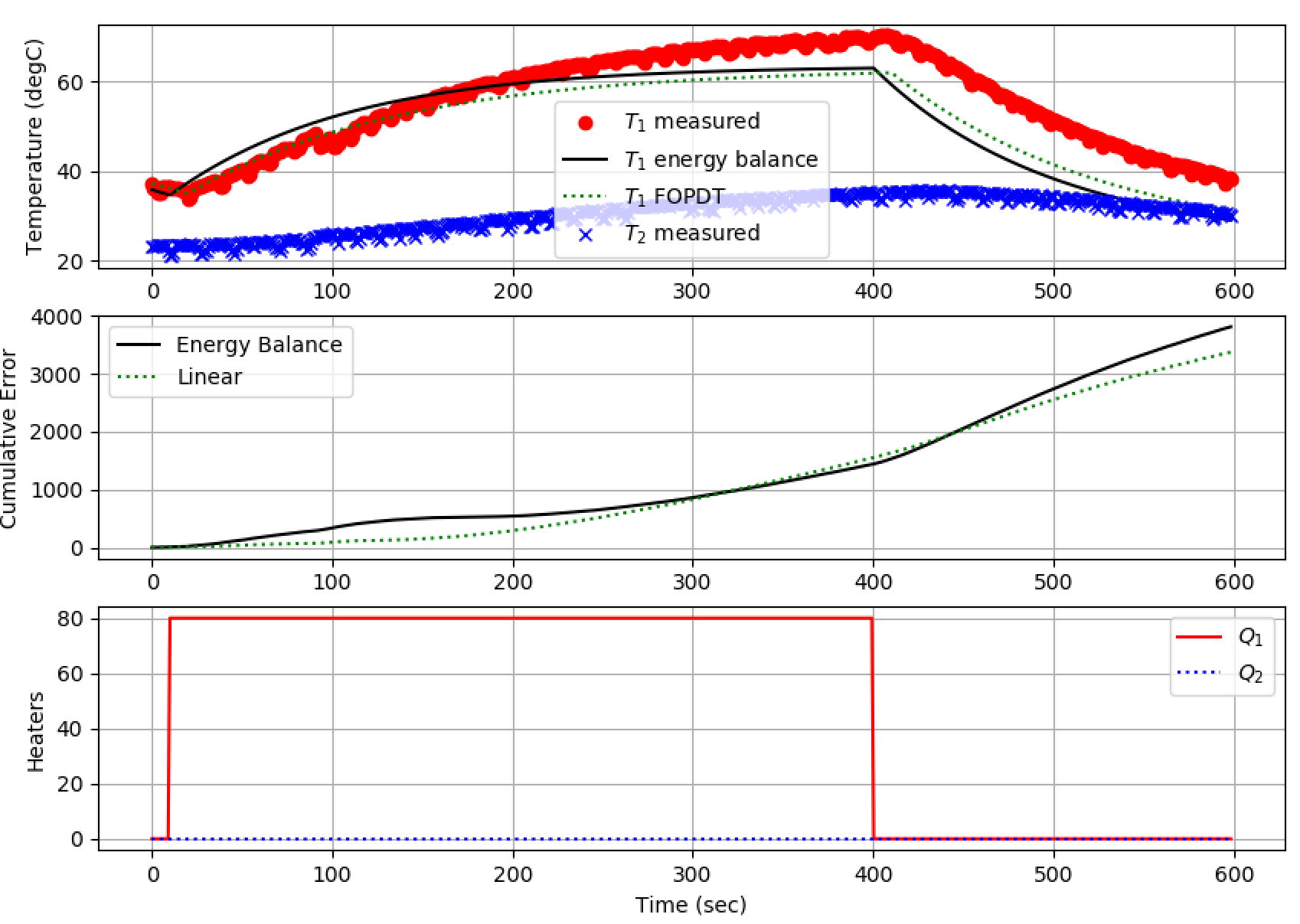
The files include a linear (FOPDT) model, a nonlinear model, and the temperature control lab interface to run the three in comparison.
The Arduino transient temperature responds similarly to the energy balance solution. Just like the physical system, this simulated system responds to changes in the heater.
import numpy as np
import time
import matplotlib.pyplot as plt
from scipy.integrate import odeint
# FOPDT model
Kp = 0.5 # degC/%
tauP = 120.0 # seconds
thetaP = 10 # seconds (integer)
Tss = 23 # degC (ambient temperature)
Qss = 0 # % heater
# define energy balance model
def heat(x,t,Q):
# Parameters
Ta = 23 + 273.15 # K
U = 10.0 # W/m^2-K
m = 4.0/1000.0 # kg
Cp = 0.5 * 1000.0 # J/kg-K
A = 12.0 / 100.0**2 # Area in m^2
alpha = 0.01 # W / % heater
eps = 0.9 # Emissivity
sigma = 5.67e-8 # Stefan-Boltzman
# Temperature State
T = x[0]
# Nonlinear Energy Balance
dTdt = (1.0/(m*Cp))*(U*A*(Ta-T) \
+ eps * sigma * A * (Ta**4 - T**4) \
+ alpha*Q)
return dTdt
# save txt file
def save_txt(t,u1,u2,y1,y2,sp1,sp2):
data = np.vstack((t,u1,u2,y1,y2,sp1,sp2)) # vertical stack
data = data.T # transpose data
top = 'Time (sec), Heater 1 (%), Heater 2 (%), ' \
+ 'Temperature 1 (degC), Temperature 2 (degC), ' \
+ 'Set Point 1 (degC), Set Point 2 (degC)'
np.savetxt('data.txt',data,delimiter=',',header=top,comments='')
# Connect to Arduino
a = tclab.TCLab()
# Turn LED on
print('LED On')
a.LED(100)
# Run time in minutes
run_time = 10.0
# Number of cycles
loops = int(60.0*run_time)
tm = np.zeros(loops)
# Temperature (K)
Tsp1 = np.ones(loops) * 23.0 # set point (degC)
T1 = np.ones(loops) * a.T1 # measured T (degC)
Tsp2 = np.ones(loops) * 23.0 # set point (degC)
T2 = np.ones(loops) * a.T2 # measured T (degC)
# Predictions
Tp = np.ones(loops) * a.T1
error_eb = np.zeros(loops)
Tpl = np.ones(loops) * a.T1
error_fopdt = np.zeros(loops)
# impulse tests (0 - 100%)
Q1 = np.ones(loops) * 0.0
Q2 = np.ones(loops) * 0.0
Q1[10:110] = 50.0 # step up for 100 sec
Q1[200:300] = 90.0 # step up for 100 sec
Q1[400:500] = 70.0 # step up for 100 sec
print('Running Main Loop. Ctrl-C to end.')
print(' Time Q1 Q2 T1 T2')
print('{:6.1f} {:6.2f} {:6.2f} {:6.2f} {:6.2f}'.format(tm[0], \
Q1[0], \
Q2[0], \
T1[0], \
T2[0]))
# Create plot
plt.figure(figsize=(10,7))
plt.ion()
plt.show()
# Main Loop
start_time = time.time()
prev_time = start_time
try:
for i in range(1,loops):
# Sleep time
sleep_max = 1.0
sleep = sleep_max - (time.time() - prev_time)
if sleep>=0.01:
time.sleep(sleep-0.01)
else:
time.sleep(0.01)
# Record time and change in time
t = time.time()
dt = t - prev_time
prev_time = t
tm[i] = t - start_time
# Read temperatures in Kelvin
T1[i] = a.T1
T2[i] = a.T2
# Simulate one time step with Energy Balance
Tnext = odeint(heat,Tp[i-1]+273.15,[0,dt],args=(Q1[i-1],))
Tp[i] = Tnext[1]-273.15
error_eb[i] = error_eb[i-1] + abs(Tp[i]-T1[i])
# Simulate one time step with FOPDT model
z = np.exp(-dt/tauP)
Tpl[i] = (Tpl[i-1]-Tss) * z \
+ (Q1[max(0,i-int(thetaP)-1)]-Qss)*(1-z)*Kp \
+ Tss
error_fopdt[i] = error_fopdt[i-1] + abs(Tpl[i]-T1[i])
# Write output (0-100)
a.Q1(Q1[i])
a.Q2(Q2[i])
# Print line of data
print('{:6.1f} {:6.2f} {:6.2f} {:6.2f} {:6.2f}'.format(tm[i], \
Q1[i], \
Q2[i], \
T1[i], \
T2[i]))
# Plot
plt.clf()
ax=plt.subplot(3,1,1)
ax.grid()
plt.plot(tm[0:i],T1[0:i],'ro',label=r'$T_1$ measured')
plt.plot(tm[0:i],Tp[0:i],'k-',label=r'$T_1$ energy balance')
plt.plot(tm[0:i],Tpl[0:i],'g:',label=r'$T_1$ FOPDT')
plt.plot(tm[0:i],T2[0:i],'bx',label=r'$T_2$ measured')
plt.ylabel('Temperature (degC)')
plt.legend(loc=2)
ax=plt.subplot(3,1,2)
ax.grid()
plt.plot(tm[0:i],error_eb[0:i],'k-',label='Energy Balance')
plt.plot(tm[0:i],error_fopdt[0:i],'g:',label='Linear')
plt.ylabel('Cumulative Error')
plt.legend(loc='best')
ax=plt.subplot(3,1,3)
ax.grid()
plt.plot(tm[0:i],Q1[0:i],'r-',label=r'$Q_1$')
plt.plot(tm[0:i],Q2[0:i],'b:',label=r'$Q_2$')
plt.ylabel('Heaters')
plt.xlabel('Time (sec)')
plt.legend(loc='best')
plt.draw()
plt.pause(0.05)
# Turn off heaters
a.Q1(0)
a.Q2(0)
# Save text file
save_txt(tm[0:i],Q1[0:i],Q2[0:i],T1[0:i],T2[0:i],Tsp1[0:i],Tsp2[0:i])
# Save figure
plt.savefig('test_Models.png')
# Allow user to end loop with Ctrl-C
except KeyboardInterrupt:
# Disconnect from Arduino
a.Q1(0)
a.Q2(0)
print('Shutting down')
a.close()
save_txt(tm[0:i],Q1[0:i],Q2[0:i],T1[0:i],T2[0:i],Tsp1[0:i],Tsp2[0:i])
plt.savefig('test_Models.png')
# Make sure serial connection still closes when there's an error
except:
# Disconnect from Arduino
a.Q1(0)
a.Q2(0)
print('Error: Shutting down')
a.close()
save_txt(tm[0:i],Q1[0:i],Q2[0:i],T1[0:i],T2[0:i],Tsp1[0:i],Tsp2[0:i])
plt.savefig('test_Models.png')
raise
Return to Temperature Control Lab Overview or Proceed to Dual Heater Modeling