TCLab FOPDT Regression
 |  |  |  |  |
|---|
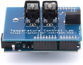
Objective: Collect step response data from the TCLab and compute parameters of an FOPDT model using an optimization method.
A single step response is required for a graphical method to obtain FOPDT parameters. A regression (optimization) approach can be used when the data cannot be fit with a graphical method. A first order plus dead time (FOPDT) model of the Temperature Control Lab (TCLab) is the following:
$$\tau_p \frac{dT'}{dt} = -T' + K_p \, Q'\left(t-\theta_p\right)$$
where `T'=T-T_{ss}` and `Q'=Q-Q_{ss}` are deviation variables with steady-state initial conditions `T_{ss}=23^oC` and `Q_{ss}=0 \%`. Perform multiple step tests with heater 1 starting at 0% for 0.5 minutes (30 seconds) and then step the heater to values between 10% and 70% for 13.5 minutes in 3-5 minute intervals. Create a plot of the temperature response over 14 minutes that shows the temperature (oC) and heater level (%). Use SimTune to collect data and optimize FOPDT parameters or use the sample source code below for generating a plot (Step_Response.png) and data file (Step_Response.csv).
import matplotlib.pyplot as plt
import pandas as pd
import tclab
import time
try:
# read Step_Response.csv if it exists
data = pd.read_csv('Step_Response.csv')
tm = data['Time'].values
Q1 = data['Q1'].values
T1 = data['T1'].values
except:
# generate data only once
n = 840 # Number of second time points (14 min)
tm = np.linspace(0,n,n+1) # Time values
lab = tclab.TCLab()
T1 = [lab.T1]
Q1 = np.zeros(n+1)
Q1[30:] = 35.0
Q1[270:] = 70.0
Q1[450:] = 10.0
Q1[630:] = 60.0
Q1[800:] = 0.0
for i in range(n):
lab.Q1(Q1[i])
time.sleep(1)
print(lab.T1)
T1.append(lab.T1)
lab.close()
# Save data file
data = np.vstack((tm,Q1,T1)).T
np.savetxt('Step_Response.csv',data,delimiter=',',\
header='Time,Q1,T1',comments='')
# Create Figure
plt.figure(figsize=(10,7))
ax = plt.subplot(2,1,1)
ax.grid()
plt.plot(tm/60.0,T1,'r.',label=r'$T_1$')
plt.ylabel(r'Temp ($^oC$)')
ax = plt.subplot(2,1,2)
ax.grid()
plt.plot(tm/60.0,Q1,'b-',label=r'$Q_1$')
plt.ylabel(r'Heater (%)')
plt.xlabel('Time (min)')
plt.legend()
plt.savefig('Step_Response.png')
plt.show()
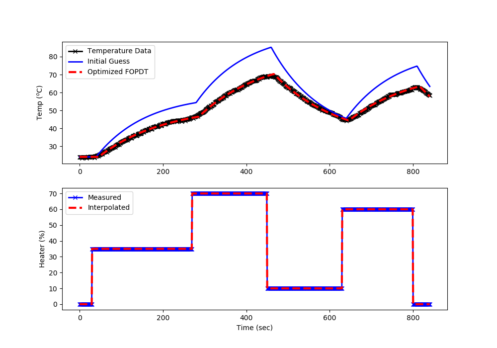
Calculate the values of `K_p`, `\tau_p`, and `\theta_p` as shown in regression of FOPDT models. Specify units for each of the parameters and compare with values from the TCLab graphical fitting FOPDT exercise.
Solution
import matplotlib.pyplot as plt
from scipy.integrate import odeint
from scipy.optimize import minimize
from scipy.interpolate import interp1d
# Import CSV data file
# Column 1 = time (t)
# Column 2 = input (u)
# Column 3 = output (yp)
data = np.loadtxt('Step_Response.csv',delimiter=',',skiprows=1)
u0 = data[0,1]
yp0 = data[0,2]
t = data[:,0].T - data[0,0]
u = data[:,1].T
yp = data[:,2].T
# specify number of steps
ns = len(t)
delta_t = t[1]-t[0]
# create linear interpolation of the u data versus time
uf = interp1d(t,u)
# define first-order plus dead-time approximation
def fopdt(y,t,uf,Km,taum,thetam):
# arguments
# y = output
# t = time
# uf = input linear function (for time shift)
# Km = model gain
# taum = model time constant
# thetam = model time constant
# time-shift u
try:
if (t-thetam) <= 0:
um = uf(0.0)
else:
um = uf(t-thetam)
except:
#print('Error with time extrapolation: ' + str(t))
um = u0
# calculate derivative
dydt = (-(y-yp0) + Km * (um-u0))/taum
return dydt
# simulate FOPDT model with x=[Km,taum,thetam]
def sim_model(x):
# input arguments
Km = x[0]
taum = x[1]
thetam = x[2]
# storage for model values
ym = np.zeros(ns) # model
# initial condition
ym[0] = yp0
# loop through time steps
for i in range(0,ns-1):
ts = [t[i],t[i+1]]
y1 = odeint(fopdt,ym[i],ts,args=(uf,Km,taum,thetam))
ym[i+1] = y1[-1]
return ym
# define objective
def objective(x):
# simulate model
ym = sim_model(x)
# calculate objective
obj = 0.0
for i in range(len(ym)):
obj = obj + (ym[i]-yp[i])**2
# return result
return obj
# initial guesses
x0 = np.zeros(3)
x0[0] = 1.0 # Km
x0[1] = 120.0 # taum
x0[2] = 10.0 # thetam
# show initial objective
print('Initial SSE Objective: ' + str(objective(x0)))
# optimize Km, taum, thetam
print('Optimizing Values...')
solution = minimize(objective,x0)
# Another way to solve: with bounds on variables
#bnds = ((0.4, 1.0), (1.0, 200.0), (0.0, 30.0))
#solution = minimize(objective,x0,bounds=bnds,method='SLSQP')
x = solution.x
# show final objective
print('Final SSE Objective: ' + str(objective(x)))
print('Kp: ' + str(x[0]))
print('taup: ' + str(x[1]))
print('thetap: ' + str(x[2]))
# calculate model with updated parameters
ym1 = sim_model(x0)
ym2 = sim_model(x)
# plot results
plt.figure(figsize=(10,7))
plt.subplot(2,1,1)
plt.plot(t,yp,'kx-',linewidth=2,label='Temperature Data')
plt.plot(t,ym1,'b-',linewidth=2,label='Initial Guess')
plt.plot(t,ym2,'r--',linewidth=3,label='Optimized FOPDT')
plt.ylabel(r'Temp ($^o$C)')
plt.legend(loc='best')
plt.subplot(2,1,2)
plt.plot(t,u,'bx-',linewidth=2)
plt.plot(t,uf(t),'r--',linewidth=3)
plt.legend(['Measured','Interpolated'],loc='best')
plt.ylabel('Heater (%)')
plt.xlabel('Time (sec)')
plt.show()