Dynamics and Control

A first-order linear system with time delay is a common empirical description of many stable dynamic processes. The equation

$$\tau_p \frac{dy(t)}{dt} = -y(t) + K_p u\left(t-\theta_p\right)$$

has variables y(t) and u(t) and three unknown parameters.

$$K_p \quad \mathrm{= Process \; gain}$$

$$\tau_p \quad \mathrm{= Process \; time \; constant}$$

$$\theta_p \quad \mathrm{= Process \; dead \; time}$$

These variables may be adjusted to match data. An explicit solution to the above equation for each time step j is:

$$y_j = e^{\frac{-\Delta\,t}{\tau_p}} \left(y_{j-1}-y_0\right) + \left(1-e^{\frac{-\Delta\,t}{\tau_p}}\right) \, K_p \, \left(u_{j-\theta_p-1}-u_0\right) + y_0$$

where `\Delta t` is the time step length, `y_0` is the initial output or steady state condition, `u_0` is the initial input or steady state condition, `y_{j-1}` and `u_{j-1}` are values from the prior step and `\theta_p` is the dead-time measured in number of time steps. When the matching process employs optimization, a model prediction is aligned with the measured values with the use of a solver. The solver often minimizes a measure of the alignment such as a sum of squared errors or sum of absolute errors. An optimization solver for Python is the SciPy.Optimize.Minimize function. Below is a tutorial on solving nonlinear optimization problems in Python.

The optimization can be applied to dynamic models as well. Below are tutorial examples using Excel or Python to adjust the parameters to fit the model predictions to data. Unlike a graphical method to fit an FOPDT model, optimization methods do not require a single step response but may include any sequence of input changes that produce a response in the output.

Fit FOPDT to Data with Excel

Fit FOPDT to Data with Python

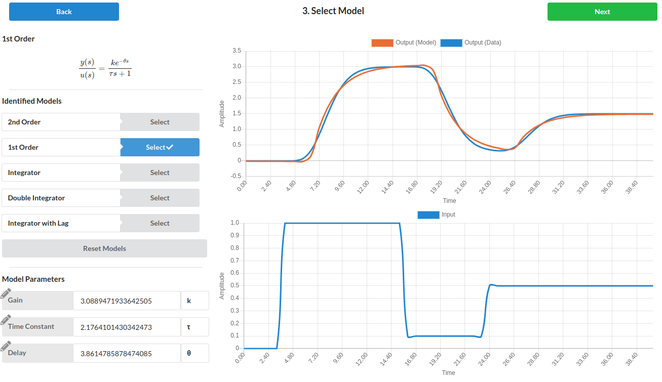
Fit FOPDT to Data with PIDTuner.com

PID Tuner generates models such as an FOPDT from data through a web-interface.

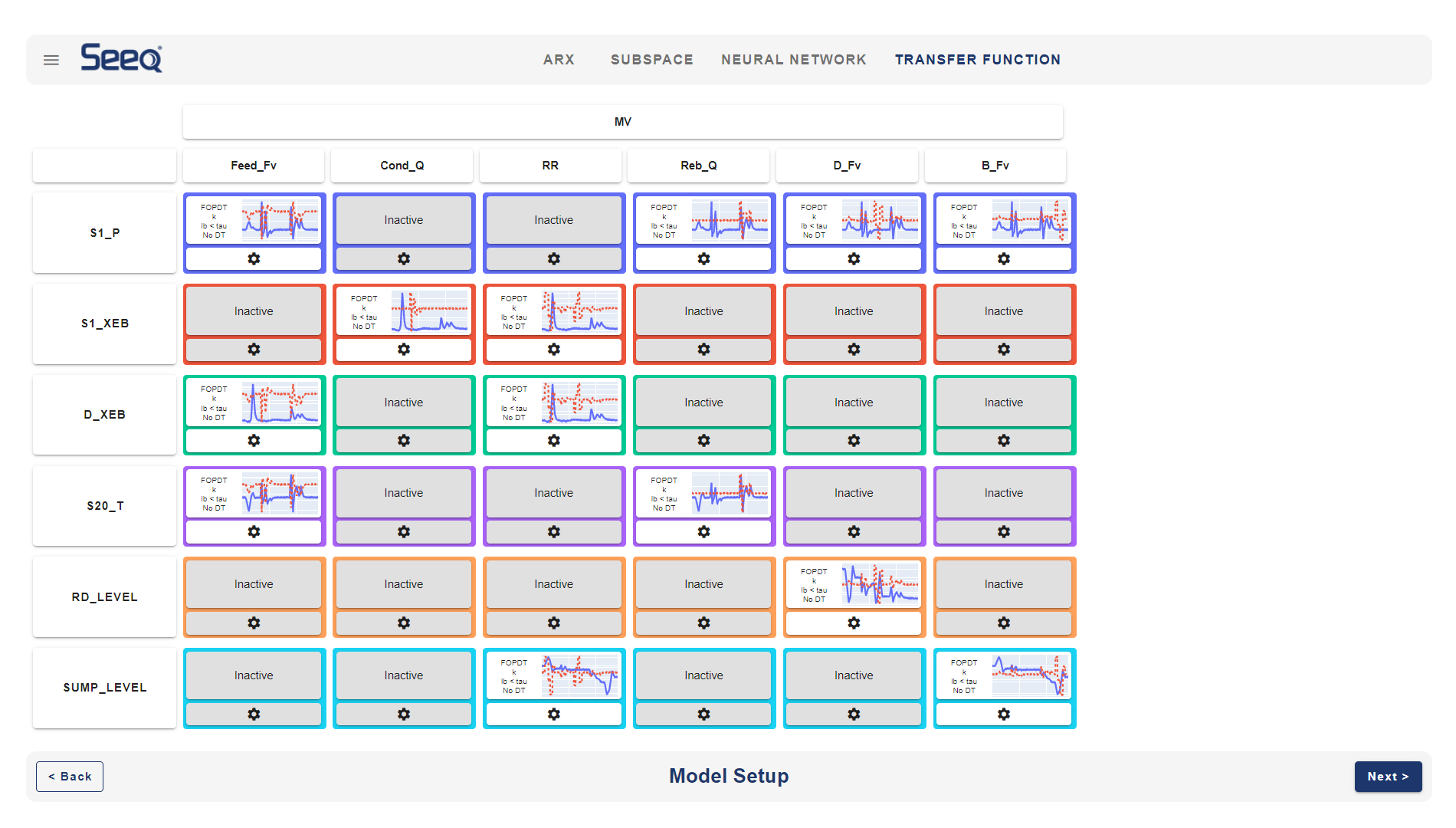
Fit Multivariate Systems with Seeq SysID

Seeq SysID is a system identification package that runs as a Seeq plugin or in a Jupyter notebook.

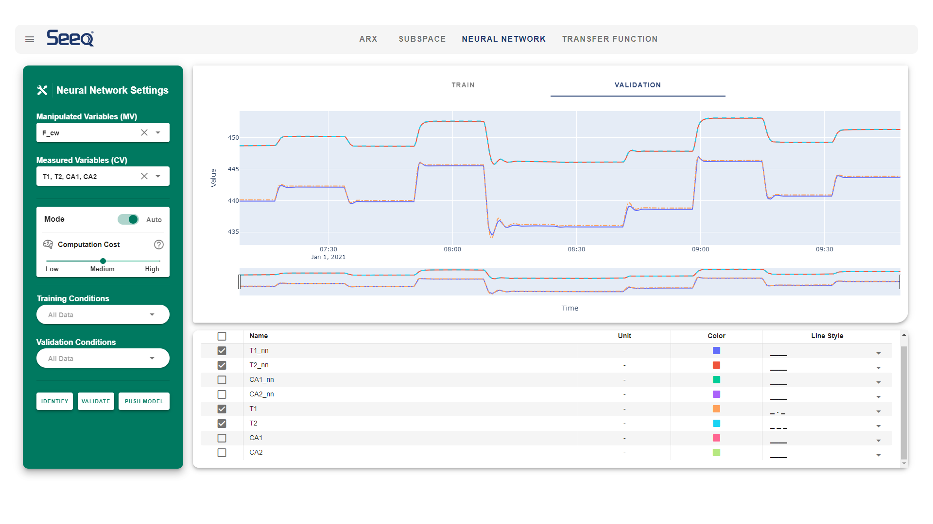
A model is created for each relationship between manipulated variable (MV) and controlled variable (CV).

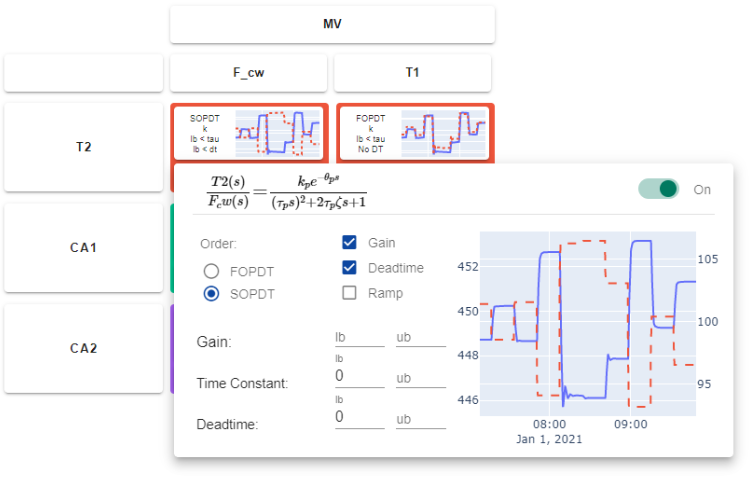
Time series, state space, Second Order Plus Dead Time (SOPDT), and FOPDT are model options. Many industrial processes use advanced control methods such as Model Predictive Control for systems with many MVs and CVs.

Graphical Fit versus Regression Fit

The graphical fitting approach is only for data with an input step response or other specialized input sequences. Use optimization to best match an FOPDT model to data with any input sequence or with more complex model. A common objective is to minimize a sum of squared error that penalizes deviation of the FOPDT model from the data. The optimization algorithm changes the parameters `K_p, \tau_p, \theta_p` to best match the data at specified time points.

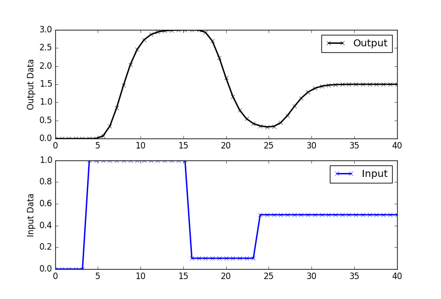
Generate Simulated Data from Model

Download data_fopdt.txt

# Generate process data as data.txt
import numpy as np
import matplotlib.pyplot as plt
from scipy.integrate import odeint

# define process model (to generate process data)
def process(y,t,n,u,Kp,taup):
    # arguments
    #  y[n] = outputs
    #  t    = time
    #  n    = order of the system  
    #  u    = input value
    #  Kp   = process gain
    #  taup = process time constant

    # equations for higher order system
    dydt = np.zeros(n)
    # calculate derivative
    dydt[0] = (-y[0] + Kp * u)/(taup/n)
    for i in range(1,n):
       dydt[i] = (-y[i] + y[i-1])/(taup/n)
    return dydt

# specify number of steps
ns = 50
# define time points
t = np.linspace(0,40,ns+1)
delta_t = t[1]-t[0]
# define input vector
u = np.zeros(ns+1)
u[5:20] = 1.0
u[20:30] = 0.1
u[30:] = 0.5

# use this function or replace yp with real process data
def sim_process_data():
    # higher order process
    n=10       # order
    Kp=3.0    # gain
    taup=5.0   # time constant
    # storage for predictions or data
    yp = np.zeros(ns+1)  # process
    for i in range(1,ns+1):
        if i==1:
            yp0 = np.zeros(n)
        ts = [delta_t*(i-1),delta_t*i]
        y = odeint(process,yp0,ts,args=(n,u[i],Kp,taup))
        yp0 = y[-1]
        yp[i] = y[1][n-1]
    return yp
yp = sim_process_data()

# Construct results and save data file
# Column 1 = time
# Column 2 = input
# Column 3 = output
data = np.vstack((t,u,yp)) # vertical stack
data = data.T              # transpose data
np.savetxt('data.txt',data,delimiter=',')

# plot results
plt.figure()
plt.subplot(2,1,1)
plt.plot(t,yp,'kx-',linewidth=2,label='Output')
plt.ylabel('Output Data')
plt.legend(loc='best')
plt.subplot(2,1,2)
plt.plot(t,u,'bx-',linewidth=2)
plt.legend(['Input'],loc='best')
plt.ylabel('Input Data')
plt.show()

[$[Get Code]]

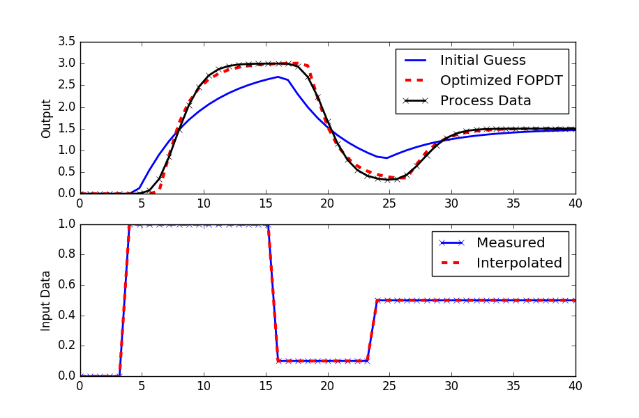
FOPDT Fit to Data