Dynamics and Control

Part A Solution: The equation is linearized by taking the partial derivative of the right hand side of the equation for both x and u.

$$\frac{\partial \left(-x^2 + \sqrt{u}\right)}{\partial x} = \alpha = -2 \, x$$

$$\frac{\partial \left(-x^2 + \sqrt{u}\right)}{\partial u} = \beta = \frac{1}{2} \frac{1}{\sqrt{u}}$$

The linearized differential equation that approximates `\frac{dx}{dt}=f(x,u)` is the following:

$$\frac{dx}{dt} = f \left(x_{ss}, u_{ss}\right) + \frac{\partial f}{\partial x}\bigg|_{x_{ss},u_{ss}} \left(x-x_{ss}\right) + \frac{\partial f}{\partial u}\bigg|_{x_{ss},u_{ss}} \left(u-u_{ss}\right)$$

Substituting in the partial derivatives results in the following differential equation:

$$\frac{dx}{dt} = 0 + \left(-2 x_{ss}\right) \left(x-x_{ss}\right) + \left(\frac{1}{2} \frac{1}{\sqrt{u_{ss}}}\right) \left(u-u_{ss}\right)$$

This is further simplified by defining new deviation variables as `x' = x - x_{ss}` and `u' = u - u_{ss}`.

$$\frac{dx'}{dt} = \alpha x' + \beta u'$$

Part B Solution: The steady state values are determined by setting `\frac{dx}{dt}=0` and solving for x.

$$0 = -x_{ss}^2 + \sqrt{u_{ss}}$$

$$x_{ss}^2 = \sqrt{16}$$

$$x_{ss} = 2$$

At steady state conditions, `frac{dx}{dt}=0` so `f (x_{ss}, u_{ss})=0` as well. Plugging in numeric values gives the simplified linear differential equation:

$$\frac{dx}{dt} = -4 \left(x-2\right) + \frac{1}{8} \left(u-16\right)$$

The partial derivatives can also be obtained from Python, either symbolically with SymPy or else numerically with SciPy.

Python program results

 -2*x
 1/(2*sqrt(u))
 Approximate Partial Derivatives
 -4.0
 0.125
 Exact Partial Derivatives
 -4.0
 0.125

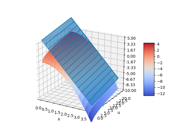
The nonlinear function for `\frac{dx}{dt}` can also be visualized with a 3D contour map. The choice of steady state conditions `x_{ss}` and `u_{ss}` produces a planar linear model that represents the nonlinear model only at a certain point. The linear model can deviate from the nonlinear model if used further away from the conditions at which the linear model is derived.

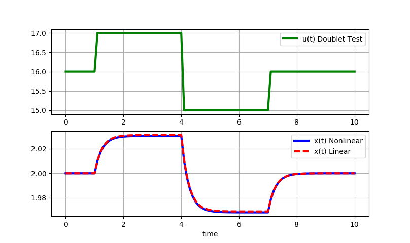
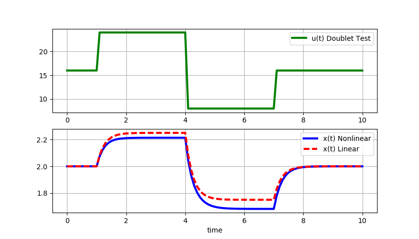
Part C Solution: The final step is to simulate a doublet test with the nonlinear and linear models.

Small step changes (+/-1): Small step changes in u lead to nearly identical responses for the linear and nonlinear solutions. The linearized model is locally accurate.

Large step changes (+/-8): As the magnitude of the doublet steps increase, the linear model deviates further from the original nonlinear equation solution.