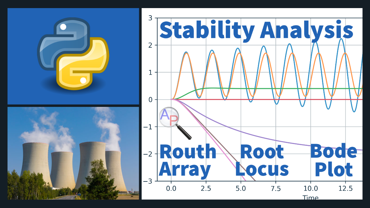
Controller Stability Analysis
 |  |  |  |
|---|
The purpose of controller stability analysis is to determine the range of controller gains between lower `K_{cL}` and upper `K_{cU}` limits that lead to a stable controller.
$$K_{cL} \le K_c \le K_{cU}$$
The principles of stability analysis presented here are general for any linear time-invariant system whether it is for controller design or for analysis of system dynamics. Several characteristics of a system in the Laplace domain can be deduced without transforming a system signal or transfer function back into the time domain. Some of the analysis relies on the roots of the transfer function denominator, also known as poles. The roots of the numerator, also known as zeros, do not affect the stability directly but can potentially cancel an unstable pole to create an overall stable system.
Converge or Diverge
A first point of analysis is whether the system converges or diverges. This is determined by analyzing the roots of the denominator of the transfer function. If any of the real parts of the roots of the denominator are positive then the system is unstable.
A simple rule to determine whether there are positive real roots is to examine the signs of the polynomial. If there are mixed signs (+ or -) then the system will be unstable because there is at least one positive real root.
Before modern computational methods, there were several methods devised to determine the stability of a system. One such approach is the Routh-Hurwitz stability criterion. The leading left edge of a table determines whether the system is stable for or any nth-degree polynomial
$$a_n s^n + a_{n-1} s^{n-1} + \cdots + a_1 s + a_0$$
The coefficients of the polynomial are placed into tabular form and additional coefficients b and c are computed from higher rows.
| `a_n` | `a_{n-2}` | `a_{n-4}` | `\ldots` |
| `a_{n-1}` | `a_{n-3}` | `a_{n-5}` | `\ldots` |
| `b_{1}=\frac{a_{n-1}a_{n-2}-a_n a_{n-3}}{a_{n-1}` | `b_{2}=\frac{a_{n-1}a_{n-4}-a_n a_{n-5}}{a_{n-1}}` | `b_{3}` | `\ldots` |
| `c_{1}=\frac{b_1 a_{n-3}-a_{n-1} b_{2}}{b_1}` | `c_{2}=\frac{b_1 a_{n-5}-a_{n-1} b_{3}}{b_1}` | `c_{3}` | `\ldots` |
| `\vdots` | `\vdots` | `\vdots` | `\ddots` |
The terms b and c are:
$$b_i=\frac{a_{n-1}\times{a_{n-2i}}-a_n\times{a_{n-2i-1}}}{a_{n-1}}$$
$$c_i=\frac{b_1\times{a_{n-2i-1}}-a_{n-1}\times{b_{i+1}}}{b_1}$$
A changing sign (+ or -) of the leading left edge `a_n`, `a_{n-1}`, `b_{1}`, `c_{1}` indicates that the system is unstable.
Several additional methods can be used to determine stability as summarized below.
| Method | Stability Condition |
| Routh Array | Leading left edge terms do not change sign |
| Root Locus Plot | All poles (roots of denominator) have negative real parts |
| Bode Plot | The response magnitude at -180 deg phase is less than one |
| Simulation | Simulate a closed loop response with increasing or decreasing controller gains until instability occurs |
In addition to analysis in the Laplace domain, stability can be determined from a model in state space form.
$$\dot x = A x + B u$$
$$y = C x + D u$$
A state space model is stable when the eigenvalues of the A matrix have negative real parts.
Oscillatory or Smooth
A second point of analysis is whether the system exhibits oscillatory or smooth behavior. If any of the roots of the denominator have an imaginary component then the system has oscillations. Imaginary roots always come in pairs with the same positive and negative imaginary values.
Final Value Theorem
The Final Value Theorem (FVT) gives the steady state gain `K_p` of a transfer function `G(s)` by taking the limit as `s \to 0`
$$K_p = \lim_{s \to 0}G(s)$$
The FVT also determines the final signal value `y_\infty` for a stable system with output `Y(s)`. Note that the Laplace variable `s` is multiplied by the signal `Y(s)` before the limit is taken.
$$y_\infty = \lim_{s \to 0} s \, Y(s)$$
The FVT may give misleading results if applied to an unstable system. It is only applicable to stable systems or signals.
Initial Value Theorem
The Initial Value Theorem (IVT) gives an initial condition of a signal by taking the limit as `s \to \infty`. Like the FVT, the Laplace variable `s` is multiplied by the signal `Y(s)` before the limit is taken.
$$y_0 = \lim_{s \to \infty} s \, Y(s)$$
Controller Stability
Controller stability analysis is finding the range of controller gains that lead to a stabilizing controller. There are multiple methods to compute this range between a lower limit `K_{cL}` and an upper limit `K_{cL}`.
$$K_{cL} \le K_c \le K_{cU}$$
This range is important to know the range of tuning values that will not lead to a destabilizing controller. With modern computational tools and powerful computers, the simulation based option is frequently used for complex systems.
Exercise
Consider a feedback control system that has the following open loop transfer function.
$$G(s) = \frac{4K_c}{(s+1)(s+2)(s+3)}$$
Determine the values of `K_c` that keep the closed loop system response stable.
Solution
First, calculate the closed loop transfer function from the open loop tranfer function.
$$G_{cl}(s)=\frac{G(s)}{1+G(s)}=\frac{\frac{4K_c}{(s+1)(s+2)(s+3)}}{1+\frac{4K_c}{(s+1)(s+2)(s+3)}}=\frac{4K_c}{(s+1)(s+2)(s+3)+4K_c}$$
$$G_{cl}(s)=\frac{4K_c}{s^3+6s^2+11s+6+4K_c}$$
Routh Array
| `a_n=1` | `a_{n-2}=11` |
| `a_{n-1}=6` | `a_{n-3}=6+4 K_c` |
| `b_{1}=\frac{66 - 6 - 4 K_c}{6}` | `b_{2}=0` |
| `c_{1}=6+4 K_c` | 0 |
The leading edge cannot change signs for the system to be stable. Therefore, the following conditions must be met:
$$a_n=1 > 0$$
$$a_{n-1}=6 > 0$$
$$b_{1}=\frac{66 - 6 - 4 K_c}{6} > 0$$
$$c_{1}=6+4 K_c > 0$$
The positive constraint on `b_1` leads to `K_c<15`. The positive constraint on `c_1` means that `K_c > -1.5`. Therefore the following ranges are acceptable for the controller stability.
$$-1.5 < K_c < 15$$
This is a more comprehensive solution than the other methods shown below because it also includes a lower bound on the controller stability limit (if a direct acting controller were inadvertently used).
Root Locus Plot
Determine where the real portion of the roots crosses to the right hand side of the plane. In this case, the real part of two roots becomes positive at `K_c=15`.
# YouTube: https://youtu.be/Y2BxAQxa0Vo
# thanks to Nikos Papadakis for the root locus slider bar
import math
import numpy as np
import matplotlib.pyplot as plt
from matplotlib.widgets import Slider, Button, RadioButtons
# open loop
num = [4.0]
den = [1.0,6.0,11.0,6.0]
def dcl(K):
return [1.0,6.0,11.0,4.0*K+6.0]
# root locus plot
n = 10000 # number of points to plot
nr = len(den)-1 # number of roots
rs = np.zeros((n,2*nr)) # store results
Kc1 = -2.0
Kc2 = 18.0
Kc = np.linspace(Kc1,Kc2,n) # Kc values
for i in range(n): # cycle through n times
roots = np.roots(dcl(Kc[i]))
for j in range(nr): # store roots
rs[i,j] = roots[j].real # store real
rs[i,j+nr] = roots[j].imag # store imaginary
# create the image
fig, ax = plt.subplots()
plt.subplots_adjust(left=0.10, bottom=0.25)
ls = []
for i in range(nr):
plt.plot(rs[:,i],rs[:,i+nr],'r.',markersize=2)
# this handle is required to update the plot
if math.isclose(rs[0,i+nr],0.0):
lbl = f'{rs[0,i]:0.2f}'
else:
lbl = f'{rs[0,i]:0.2f}, {rs[0,i+nr]:0.2f}i'
l, = plt.plot(rs[0,i],rs[0,i+nr], 'ks', markersize=5,label=lbl)
ls.append(l)
leg = plt.legend(loc='best')
plt.xlabel('Root (real)')
plt.ylabel('Root (imag)')
plt.grid(b=True, which='major', color='b', linestyle='-',alpha=0.5)
plt.grid(b=True, which='minor', color='r', linestyle='--',alpha=0.5)
plt.xlim([-4.0,0.5])
#plt.ylim([-4.0,4.0])
# slider creation
axcolor = 'lightgoldenrodyellow'
axKc = plt.axes([0.10, 0.1, 0.80, 0.03], facecolor=axcolor)
sKc = Slider(axKc, 'Kc', Kc1, Kc2, valinit=0, valstep=0.1)
def update(val):
Kc_val= sKc.val
indx = (np.abs(Kc-Kc_val)).argmin()
for i in range(nr):
ls[i].set_ydata(rs[indx,i+nr])
ls[i].set_xdata(rs[indx,i])
if math.isclose(rs[indx,i+nr],0.0):
lbl = f'{rs[indx,i]:0.2f}'
else:
lbl = f'{rs[indx,i]:0.2f}, {rs[indx,i+nr]:0.2f}i'
leg.texts[i].set_text(lbl)
fig.canvas.draw_idle()
sKc.on_changed(update)
resetax = plt.axes([0.8, 0.025, 0.1, 0.04])
button = Button(resetax, 'Reset', color=axcolor, hovercolor='0.975')
def reset(event):
sKc.reset()
button.on_clicked(reset)
plt.show()
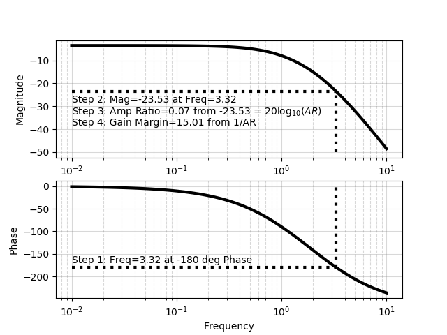
Bode Plot
Determine the gain margin at -180o phase. The magnitude at -180o phase is about -23 dB. With `-23 = 20 log_{10} (AR)`, the gain margin is `1/{AR}` and approximately equal to 15. This is the upper bound on the controller gain to keep the system stable. This answer agrees with the root locus plot solution.
from scipy import signal
import matplotlib.pyplot as plt
from scipy.interpolate import interp1d
# open loop
num = [4.0]
den = [1.0,6.0,11.0,6.0]
sys = signal.TransferFunction(num, den)
t1,y1 = signal.step(sys)
# closed loop
Kc = 1.0
num = [4.0*Kc]
den = [1.0,6.0,11.0,4.0*Kc+6.0]
sys2 = signal.TransferFunction(num, den)
t2,y2 = signal.step(sys2)
plt.figure(1)
plt.subplot(2,1,1)
plt.plot(t1,y1,'k-')
plt.legend(['Open Loop'],loc='best')
plt.subplot(2,1,2)
plt.plot(t2,y2,'r--')
plt.legend(['Closed Loop'],loc='best')
plt.xlabel('Time')
# root locus plot
n = 1000 # number of points to plot
nr = 3 # number of roots
rs = np.zeros((n,2*nr)) # store results
Kc = np.logspace(-2,2,n) # Kc values
for i in range(n): # cycle through n times
den = [1.0,6.0,11.0,4.0*Kc[i]+6.0] # polynomial
roots = np.roots(den) # find roots
for j in range(nr): # store roots
rs[i,j] = roots[j].real # store real
rs[i,j+nr] = roots[j].imag # store imaginary
plt.figure(2)
plt.subplot(2,1,1)
plt.xlabel('Root (real)')
plt.ylabel('Root (imag)')
plt.grid(b=True, which='major', color='b', linestyle='-')
plt.grid(b=True, which='minor', color='r', linestyle='--')
for i in range(nr):
plt.plot(rs[:,i],rs[:,i+nr],'.')
plt.subplot(2,1,2)
plt.plot([Kc[0],Kc[-1]],[0,0],'k-')
for i in range(3):
plt.plot(Kc,rs[:,i],'.')
plt.ylabel('Root (real part)')
plt.xlabel('Controller Gain (Kc)')
# bode plot
w,mag,phase = signal.bode(sys)
# compute the gain margin
mag_f = interp1d(phase, mag)
mag_f(-180) # magnitude at -180 degrees
AR = 10**(mag_f(-180)/20.0)
print('Gain Margin : {}'.format(1.0/AR))
plt.figure(3)
plt.subplot(2,1,2) # bottom plot
plt.semilogx(w,phase,'k-',linewidth=3)
plt.grid(b=True, which='major', color='grey', alpha=0.3, linestyle='-')
plt.grid(b=True, which='minor', color='grey', alpha=0.3, linestyle='--')
# show graphical gain margin calc on plot
w_i = interp1d(phase,w)
mag_i = interp1d(w,mag)
wcr = w_i(-180.0)
# gain ratio 1: show freq that intersects at -180 phase
plt.semilogx([0.01,wcr],[-180,-180], 'k:', lw=3)
# gain ratio 2: show mag at that frequency
plt.semilogx([wcr,wcr],[-180,0], 'k:', lw=3)
plt.text(0.01,-170,f'Step 1: Freq={wcr:0.2f} at -180 deg Phase')
plt.ylabel('Phase')
plt.xlabel('Frequency')
plt.subplot(2,1,1) # top plot
plt.semilogx(w,mag,'k-',linewidth=3)
plt.grid(b=True, which='major', color='grey', alpha=0.3, linestyle='-')
plt.grid(b=True, which='minor', color='grey', alpha=0.3, linestyle='--')
plt.ylabel('Magnitude')
# gain ratio 3:
plt.semilogx([wcr,wcr],[-50,mag_i(wcr)], 'k:', lw=3)
# gain ratio 4:
plt.semilogx([0.01,wcr],[mag_i(wcr),mag_i(wcr)], 'k:', lw=3)
plt.text(0.01,mag_i(wcr)-5,f'Step 2: Mag={mag_i(wcr):0.2f} at Freq={wcr:0.2f}')
AR = 10**(mag_i(wcr)/20.0)
plt.text(0.01,mag_i(wcr)-10,f'Step 3: Amp Ratio={AR:0.2f} ' + \
f'from {mag_i(wcr):0.2f} = ' + \
'20$\log_{10}(AR)$')
plt.text(0.01,mag_i(wcr)-15,f'Step 4: Gain Margin={1.0/AR:0.2f} ' + \
f'from 1/AR')
plt.show()
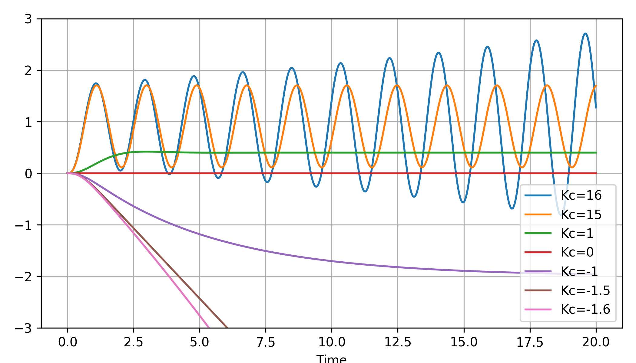
Stability Simulation
A simulation of the closed loop system verifies the stability limits of -1.5 (lower) and 15 (upper).
from scipy import signal
import matplotlib.pyplot as plt
def sim(Kc):
tm = np.linspace(0,20,1000)
num = [4.0*Kc]
den = [1,6,11,6+4*Kc]
sys = signal.TransferFunction(num, den)
t,y = signal.step(sys,T=tm)
return t,y
plt.figure(figsize=(7,4))
for K in [16,15,1,0,-1,-1.5,-1.6]:
t,y = sim(K)
plt.plot(t,y,label='Kc='+str(K))
plt.legend(); plt.grid()
plt.ylim([-3,3]); plt.tight_layout()
plt.xlabel('Time')
plt.show()
Numerical methods can simulate nonlinear systems, constraints, and other realistic system characteristics that cannot be analyzed with the linear methods of Routh Arrays, Root Locus, or Bode Plots.
Additional Root Locus Example
Find the stability limit for `K_c` for the following closed-loop transfer function.
$$\frac{1}{\left(x^2+x+1\right)\left(x+1\right)^2-2K_c}$$


Assignment
See Stability Analysis Exercises