Optimization Method: SOPDT to Data
 |  |  |  |
|---|
A second-order linear system with time delay is an empirical description of potentially oscillating dynamic processes. The equation
$$\tau_s^2 \frac{d^2y}{dt^2} + 2 \zeta \tau_s \frac{dy}{dt} + y = K_p \, u\left(t-\theta_p \right)$$
has output y(t) and input u(t) and four unknown parameters. The four parameters are the gain `K_p`, damping factor `\zeta`, second order time constant `\tau_s`, and dead time `\theta_p`.
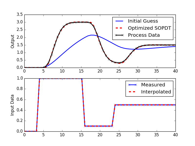
An alternative to the graphical fitting approach is to use optimization to best match an SOPDT model to data. A common objective is to minimize a sum of squared error that penalizes deviation of the SOPDT model from the data. The optimization algorithm changes the parameters `(K_p, \tau_p, \zeta, \theta_p)` to best match the data at specified time points.
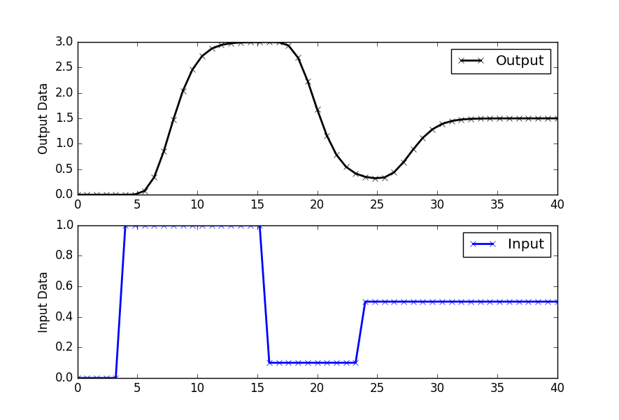
Generate Simulated Data from Model

import numpy as np
import matplotlib.pyplot as plt
from scipy.integrate import odeint
# define process model (to generate process data)
def process(y,t,n,u,Kp,taup):
# arguments
# y[n] = outputs
# t = time
# n = order of the system
# u = input value
# Kp = process gain
# taup = process time constant
# equations for higher order system
dydt = np.zeros(n)
# calculate derivative
dydt[0] = (-y[0] + Kp * u)/(taup/n)
for i in range(1,n):
dydt[i] = (-y[i] + y[i-1])/(taup/n)
return dydt
# specify number of steps
ns = 50
# define time points
t = np.linspace(0,40,ns+1)
delta_t = t[1]-t[0]
# define input vector
u = np.zeros(ns+1)
u[5:20] = 1.0
u[20:30] = 0.1
u[30:] = 0.5
# use this function or replace yp with real process data
def sim_process_data():
# higher order process
n=10 # order
Kp=3.0 # gain
taup=5.0 # time constant
# storage for predictions or data
yp = np.zeros(ns+1) # process
for i in range(1,ns+1):
if i==1:
yp0 = np.zeros(n)
ts = [delta_t*(i-1),delta_t*i]
y = odeint(process,yp0,ts,args=(n,u[i],Kp,taup))
yp0 = y[-1]
yp[i] = y[1][n-1]
return yp
yp = sim_process_data()
# Construct results and save data file
# Column 1 = time
# Column 2 = input
# Column 3 = output
data = np.vstack((t,u,yp)) # vertical stack
data = data.T # transpose data
np.savetxt('data.txt',data,delimiter=',',comments='',header='time,u,y')
# plot results
plt.figure()
plt.subplot(2,1,1)
plt.plot(t,yp,'kx-',linewidth=2,label='Output')
plt.ylabel('Output Data')
plt.legend(loc='best')
plt.subplot(2,1,2)
plt.plot(t,u,'bx-',linewidth=2)
plt.legend(['Input'],loc='best')
plt.ylabel('Input Data')
plt.show()
SOPDT Fit to Data
import pandas as pd
import matplotlib.pyplot as plt
from scipy.integrate import odeint
from scipy.optimize import minimize
from scipy.interpolate import interp1d
import warnings
# Import CSV data file
# Column 1 = time (t)
# Column 2 = input (u)
# Column 3 = output (yp)
url = 'http://apmonitor.com/pdc/uploads/Main/data_fopdt.txt'
data = pd.read_csv(url)
t = data['time'].values - data['time'].values[0]
u = data['u'].values
yp = data['y'].values
u0 = u[0]
y0 = yp[0]
xp0 = yp[0]
# specify number of steps
ns = len(t)
delta_t = t[1]-t[0]
# create linear interpolation of the u data versus time
uf = interp1d(t,u)
def sopdt(x,t,uf,Kp,taus,zeta,thetap):
# Kp = process gain
# taus = second order time constant
# zeta = damping factor
# thetap = model time delay
# ts^2 dy2/dt2 + 2 zeta taus dydt + y = Kp u(t-thetap)
# time-shift u
try:
if (t-thetap) <= 0:
um = uf(0.0)
else:
um = uf(t-thetap)
except:
# catch any error
um = u0
# two states (y and y')
y = x[0] - y0
dydt = x[1]
dy2dt2 = (-2.0*zeta*taus*dydt - y + Kp*(um-u0))/taus**2
return [dydt,dy2dt2]
# simulate model with x=[Km,taum,thetam]
def sim_model(x):
# input arguments
Kp = x[0]
taus = x[1]
zeta = x[2]
thetap = x[3]
# storage for model values
xm = np.zeros((ns,2)) # model
# initial condition
xm[0] = xp0
# loop through time steps
for i in range(0,ns-1):
ts = [t[i],t[i+1]]
inputs = (uf,Kp,taus,zeta,thetap)
# turn off warnings
with warnings.catch_warnings():
warnings.simplefilter("ignore")
# integrate SOPDT model
x = odeint(sopdt,xm[i],ts,args=inputs)
xm[i+1] = x[-1]
y = xm[:,0]
return y
# define objective
def objective(x):
# simulate model
ym = sim_model(x)
# calculate objective
obj = 0.0
for i in range(len(ym)):
obj = obj + (ym[i]-yp[i])**2
# return result
return obj
# initial guesses
p0 = np.zeros(4)
p0[0] = 3 # Kp
p0[1] = 5.0 # taup
p0[2] = 1.0 # zeta
p0[3] = 2.0 # thetap
# show initial objective
print('Initial SSE Objective: ' + str(objective(p0)))
# optimize Kp, taus, zeta, thetap
solution = minimize(objective,p0)
# with bounds on variables
#no_bnd = (-1.0e10, 1.0e10)
#low_bnd = (0.01, 1.0e10)
#bnds = (no_bnd, low_bnd, low_bnd, low_bnd)
#solution = minimize(objective,p0,method='SLSQP',bounds=bnds)
p = solution.x
# show final objective
print('Final SSE Objective: ' + str(objective(p)))
print('Kp: ' + str(p[0]))
print('taup: ' + str(p[1]))
print('zeta: ' + str(p[2]))
print('thetap: ' + str(p[3]))
# calculate model with updated parameters
ym1 = sim_model(p0)
ym2 = sim_model(p)
# plot results
plt.figure()
plt.subplot(2,1,1)
plt.plot(t,ym1,'b-',linewidth=2,label='Initial Guess')
plt.plot(t,ym2,'r--',linewidth=3,label='Optimized SOPDT')
plt.plot(t,yp,'k--',linewidth=2,label='Process Data')
plt.ylabel('Output')
plt.legend(loc='best')
plt.subplot(2,1,2)
plt.plot(t,u,'bx-',linewidth=2)
plt.plot(t,uf(t),'r--',linewidth=3)
plt.legend(['Measured','Interpolated'],loc='best')
plt.ylabel('Input Data')
plt.savefig('results.png')
plt.show()
import pandas as pd
from gekko import GEKKO
import matplotlib.pyplot as plt
# Import CSV data file
# Column 1 = time (t)
# Column 2 = input (u)
# Column 3 = output (y)
url = 'http://apmonitor.com/pdc/uploads/Main/data_sopdt.txt'
data = pd.read_csv(url)
t = data['time'].values - data['time'].values[0]
u = data['u'].values
y = data['y'].values
m = GEKKO(remote=False)
m.time = t; time = m.Var(0); m.Equation(time.dt()==1)
K = m.FV(2,lb=0,ub=10); K.STATUS=1
tau = m.FV(3,lb=1,ub=200); tau.STATUS=1
theta_ub = 30 # upper bound to dead-time
theta = m.FV(0,lb=0,ub=theta_ub); theta.STATUS=1
zeta = m.FV(1,lb=0.1,ub=3); zeta.STATUS=1
# add extrapolation points
td = np.concatenate((np.linspace(-theta_ub,min(t)-1e-5,5),t))
ud = np.concatenate((u[0]*np.ones(5),u))
# create cubic spline with t versus u
uc = m.Var(u); tc = m.Var(t); m.Equation(tc==time-theta)
m.cspline(tc,uc,td,ud,bound_x=False)
ym = m.Param(y); yp = m.Var(y); xp = m.Var(y)
m.Equation(xp==yp.dt())
m.Equation((tau**2)*xp.dt()+2*zeta*tau*yp.dt()+yp==K*(uc-u[0]))
m.Minimize((yp-ym)**2)
m.options.IMODE=5
m.solve(disp=False)
print('Kp: ', K.value[0])
print('taup: ', tau.value[0])
print('thetap: ', theta.value[0])
print('zetap: ', zeta.value[0])
# plot results
plt.figure()
plt.subplot(2,1,1)
plt.plot(t,y,'k.-',lw=2,label='Process Data')
plt.plot(t,yp.value,'r--',lw=2,label='Optimized SOPDT')
plt.ylabel('Output')
plt.legend()
plt.subplot(2,1,2)
plt.plot(t,u,'b.-',lw=2,label='u')
plt.legend()
plt.ylabel('Input')
plt.show()
Assignment