Dynamic Optimization
In order to apply dynamic optimization methods we must have a dynamic model to optimize. Obtaining a good dynamic model of the design problem is the most important step. A static model is often developed first and can often be augmented to include dynamic elements that relate how the system evolves with time. In this section we discuss some modeling concepts for dynamic systems that can help you develop models for optimization. We also discuss the formulation objectives, constraints, and dynamic data sets. See the Dynamic Optimization Course for additional content.
Fitting Physical Models to Experimental Data
Dynamic models are often constructed with physical models and tuned with experimental data. Physical models are based on the underlying physical principles that govern the problem and result from expressions such as a force or momentum balance and may include quantities such as velocity, acceleration, and position. Other quantities of interest may include anything that changes with respect to time such as reactor composition, temperature, mole fraction, etc. Models likely contain both physical and experimental elements. We will discuss how to reconcile experimental data with the physical model through parameter estimation. A final activity will be to use the physical model to then optimize a particular objective.
Introduction to Dynamic Modeling with MATLAB and Python
This 5 minute tutorial gives step-by-step instructions on how to simulate dynamic systems. Dynamic systems may have differential and algebraic equations (DAEs) or just differential equations (ODEs) that cause a time evolution of the response. The tutorial covers the same problem in both MATLAB and Python.
Simulate Dynamic Data with Python and MATLAB
This next tutorial covers how to simulate changing inputs over a time horizon with a dynamic model. The inputs change at regular intervals, causing a time varying response in the output. The same simulation is produced in both MATLAB and Python.
Insulin Injection Optimization for Diabetic Blood Glucose Regulation
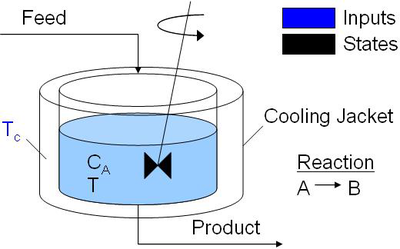
Reduce Pollution from an Exothermic Reactor
The objective is to reduce the concentration of the pollution from an exothermic reactor without exceeding an upper temperature limit. Python, MATLAB, and Simulink simulations are available for download at the link below.
Simulink Estimation and Control with APM
The following files are a Simulink example of dynamic estimation and dynamic optimization. Separate blocks run the estimation and control algorithms for Model Predictive Control (MPC) with constrained nonlinear programming.
