TCLab PI Control Tuning
 |  |  |  |
|---|
Objective: For PI control of the TCLab, use the IMC and ITAE tuning correlations and compare the integral absolute error difference between setpoint and measured temperature for a setpoint change from 23 to 60 oC.
Common tuning correlations for PI control are the IMC (Internal Model Control) and ITAE (Integral of Time-weighted Absolute Error) methods. Use the IMC and ITAE setpoint tracking tuning correlations with FOPDT parameters (`K_c`, `\tau_p`, `\theta_p`) determined from the TCLab graphical fitting or TCLab regression exercises.
IMC Aggressive Tuning
$$\tau_c = \max \left( 0.1 \tau_p, 0.8 \theta_p \right)$$
$$K_c = \frac{1}{K_p}\frac{\tau_p}{\left( \theta_p + \tau_c \right)} \quad \quad \tau_I = \tau_p$$
ITAE Tuning
$$K_c = \frac{0.586}{K_p}\left(\frac{\theta_p}{\tau_p}\right)^{-0.916} \quad \tau_I = \frac{\tau_p}{1.03-0.165\left(\theta_p/\tau_p\right)}$$
Fill in the values of `K_c`, `\tau_I`, and the PI equation in the code below. Run both tuning correlations separately with the TCLab to determine the integral absolute error difference between the setpoint and measured temperature.
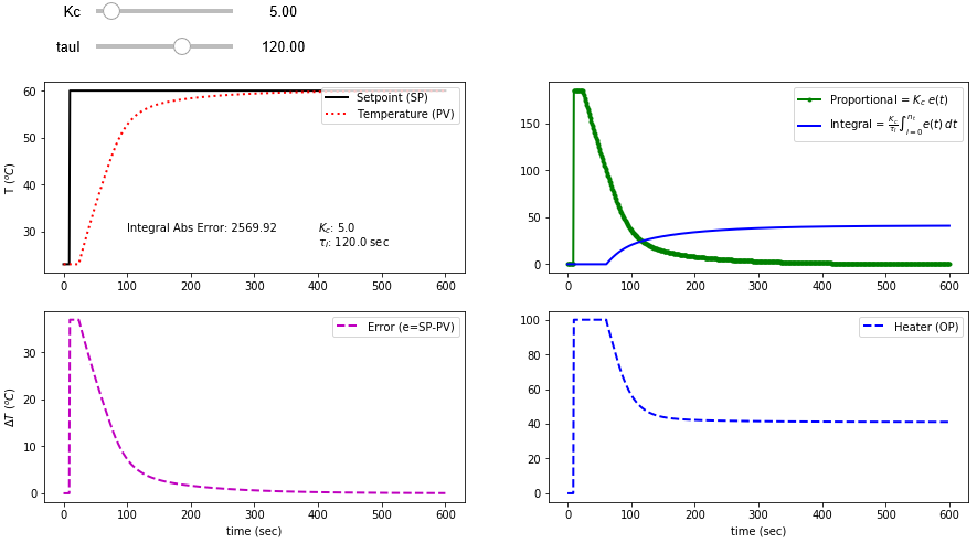
PI Control Simulator
A PI Control simulator can be used to anticipate the control performance with changes in control tuning parameters, `K_c` and `\tau_I`. The IMC and ITAE recommended values can be tested before implementing the closed loop control with the TCLab. Adjust the slider bars in the Jupyter notebook to see the updated plots and calculated integral absolute error.


from IPython.display import clear_output
import matplotlib.pyplot as plt
from scipy.integrate import odeint
import ipywidgets as wg
from IPython.display import display
n = 601 # time points to plot
tf = 600.0 # final time
# TCLab FOPDT
Kp = 0.9
taup = 175.0
thetap = 15.0
def process(y,t,u):
dydt = (1.0/taup) * (-(y-23.0) + Kp * u)
return dydt
def pidPlot(Kc,tauI):
t = np.linspace(0,tf,n) # create time vector
P = np.zeros(n) # initialize proportional term
I = np.zeros(n) # initialize integral term
e = np.zeros(n) # initialize error
OP = np.zeros(n) # initialize controller output
PV = np.ones(n)*23.0 # initialize process variable
SP = np.ones(n)*23.0 # initialize setpoint
SP[10:] = 60.0 # step up
y0 = 23.0 # initial condition
iae = 0.0
# loop through all time steps
for i in range(1,n):
# simulate process for one time step
ts = [t[i-1],t[i]] # time interval
y = odeint(process,y0,ts,args=(OP[max(0,i-int(thetap))],))
y0 = y[1] # record new initial condition
iae += np.abs(SP[i]-y0[0])
# calculate new OP with PID
PV[i] = y[1] # record PV
e[i] = SP[i] - PV[i] # calculate error = SP - PV
dt = t[i] - t[i-1] # calculate time step
P[i] = Kc * e[i] # calculate proportional term
I[i] = I[i-1] + (Kc/tauI) * e[i] * dt # calculate integral term
OP[i] = P[i] + I[i] # calculate new controller output
if OP[i]>=100:
OP[i] = 100.0
I[i] = I[i-1] # reset integral
if OP[i]<=0:
OP[i] = 0.0
I[i] = I[i-1] # reset integral
# plot PID response
plt.figure(1,figsize=(15,7))
clear_output()
plt.subplot(2,2,1)
plt.plot(t,SP,'k-',linewidth=2,label='Setpoint (SP)')
plt.plot(t,PV,'r:',linewidth=2,label='Temperature (PV)')
plt.ylabel(r'T $(^oC)$')
plt.text(100,30,'Integral Abs Error: ' + str(np.round(iae,2)))
plt.text(400,30,r'$K_c$: ' + str(np.round(Kc,0)))
plt.text(400,27,r'$\tau_I$: ' + str(np.round(tauI,0)) + ' sec')
plt.legend(loc=1)
plt.subplot(2,2,2)
plt.plot(t,P,'g.-',linewidth=2,label=r'Proportional = $K_c \; e(t)$')
plt.plot(t,I,'b-',linewidth=2,label=r'Integral = ' + \
r'$\frac{K_c}{\tau_I} \int_{i=0}^{n_t} e(t) \; dt $')
plt.legend(loc='best')
plt.subplot(2,2,3)
plt.plot(t,e,'m--',linewidth=2,label='Error (e=SP-PV)')
plt.ylabel(r'$\Delta T$ $(^oC)$')
plt.legend(loc='best')
plt.xlabel('time (sec)')
plt.subplot(2,2,4)
plt.plot(t,OP,'b--',linewidth=2,label='Heater (OP)')
plt.legend(loc='best')
plt.xlabel('time (sec)')
plt.show()
Kc_slide = wg.FloatSlider(value=5.0,min=0.0,max=50.0,step=1.0)
tauI_slide = wg.FloatSlider(value=120.0,min=20.0,max=180.0,step=5.0)
wg.interact(pidPlot, Kc=Kc_slide, tauI=tauI_slide)
print('PID Simulator: Adjust Kc and tauI for lowest Integral Abs Error')
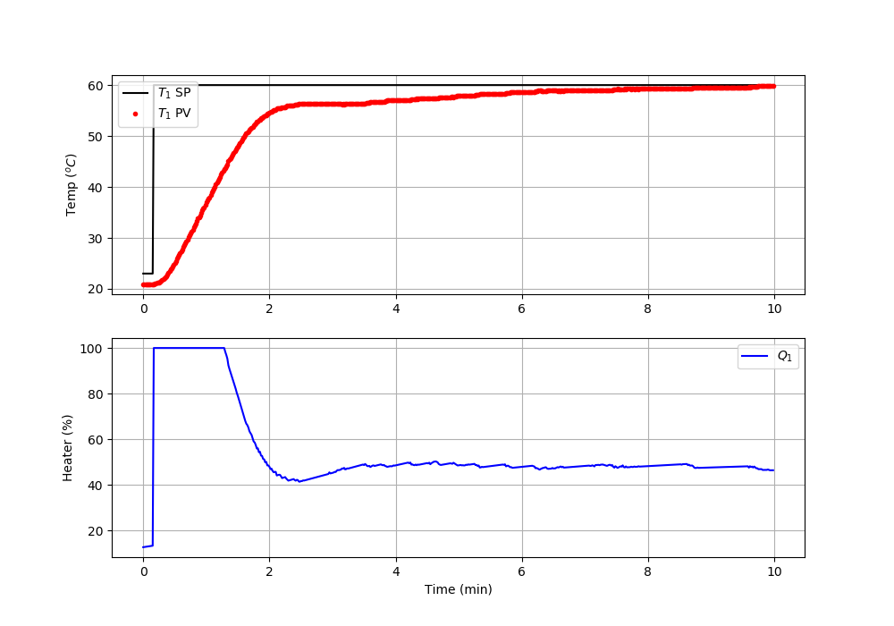
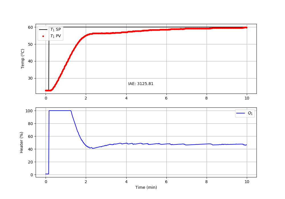
PI Control Validation
A PI control script is available for testing IMC and ITAE recommended parameters. Input the `K_c` and `\tau_I` values from the tuning correlation to test with the TCLab.
tauI = 120
import matplotlib.pyplot as plt
import tclab
import time
# PI Parameters
Kc = 5
tauI = 120
tauD = 0 # no derivative term
print('Kc: ' + str(Kc))
print('tauI: ' + str(tauI))
#------------------------
# PID Controller Function
#------------------------
# sp = setpoint
# pv = current temperature
# pv_last = prior temperature
# ierr = integral error
# dt = time increment between measurements
# outputs ---------------
# op = output of the PID controller
# P = proportional contribution
# I = integral contribution
# D = derivative contribution
def pid(sp,pv,pv_last,ierr,dt):
# Parameters in terms of PID coefficients
KP = Kc
KI = Kc/tauI
KD = Kc*tauD
# ubias for controller (initial heater)
op0 = 0
# upper and lower bounds on heater level
ophi = 100
oplo = 0
# calculate the error
error = sp-pv
# calculate the integral error
ierr = ierr + KI * error * dt
# calculate the measurement derivative
dpv = (pv - pv_last) / dt
# calculate the PID output
P = KP * error
I = ierr
D = -KD * dpv
op = op0 + P + I + D
# implement anti-reset windup
if op < oplo or op > ophi:
I = I - KI * error * dt
# clip output
op = max(oplo,min(ophi,op))
# return the controller output and PID terms
return [op,P,I,D]
n = 600 # Number of second time points (10 min)
tm = np.linspace(0,n-1,n) # Time values
lab = tclab.TCLab()
T1 = np.zeros(n)
Q1 = np.zeros(n)
# step setpoint from 23.0 to 60.0 degC
SP1 = np.ones(n)*23.0
SP1[10:] = 60.0
Q1_bias = 0.0
ierr = 0.0
for i in range(n):
# record measurement
T1[i] = lab.T1
# --------------------------------------------------
# call PID controller function to change Q1[i]
# --------------------------------------------------
[Q1[i],P,ierr,D] = pid(SP1[i],T1[i],T1[max(0,i-1)],ierr,1.0)
lab.Q1(Q1[i])
if i%20==0:
print(' Heater, Temp, Setpoint')
print(f'{Q1[i]:7.2f},{T1[i]:7.2f},{SP1[i]:7.2f}')
# wait for 1 sec
time.sleep(1)
lab.close()
# Save data file
data = np.vstack((tm,Q1,T1,SP1)).T
np.savetxt('PI_control.csv',data,delimiter=',',\
header='Time,Q1,T1,SP1',comments='')
# Create Figure
plt.figure(figsize=(10,7))
ax = plt.subplot(2,1,1)
ax.grid()
plt.plot(tm/60.0,SP1,'k-',label=r'$T_1$ SP')
plt.plot(tm/60.0,T1,'r.',label=r'$T_1$ PV')
plt.ylabel(r'Temp ($^oC$)')
plt.legend(loc=2)
ax = plt.subplot(2,1,2)
ax.grid()
plt.plot(tm/60.0,Q1,'b-',label=r'$Q_1$')
plt.ylabel(r'Heater (%)')
plt.xlabel('Time (min)')
plt.legend(loc=1)
plt.savefig('PI_Control.png')
plt.show()
Optimization of PI Tuning (not required)
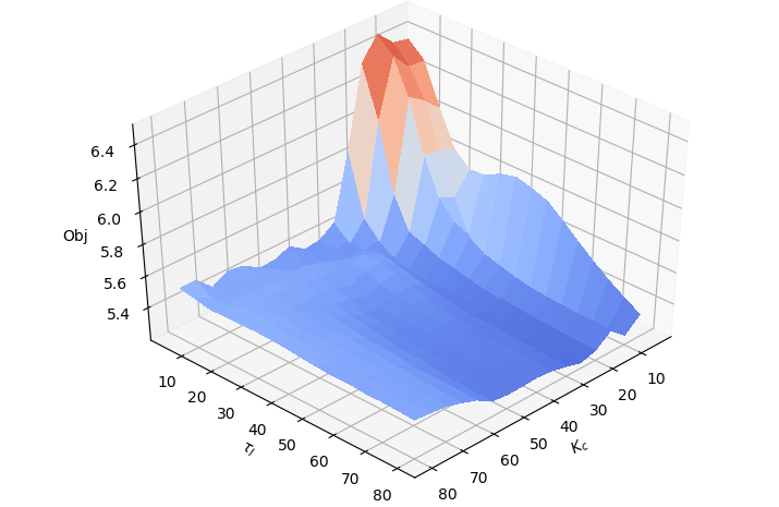
Optimization is another method for tuning PID controllers. Using closed-loop data and a model of the process (e.g. FOPDT or ARX), candidate PID parameters can be simulated to determine the best performance. The following 3D plot is the average integral absolute error for temperature and heater movements for the TCLab with `K_c` and `\tau_I` parameters. The lowest objective is the best performance at `K_c`=10.0 and `\tau_I`=55.0 sec. More information on optimization is provided in the Design Optimization Course and the Machine Learning and Dynamic Optimization Course.
Reference
Park, J., Patterson, C., Kelly, J., Hedengren, J.D., Closed-Loop PID Re-Tuning in a Digital Twin By Re-Playing Past Setpoint and Load Disturbance Data, AIChE Spring Meeting, New Orleans, LA, April 2019. Abstract
Solutions
import matplotlib.pyplot as plt
import tclab
import time
# process model
Kp = 0.9
taup = 175.0
thetap = 15.0
# -----------------------------
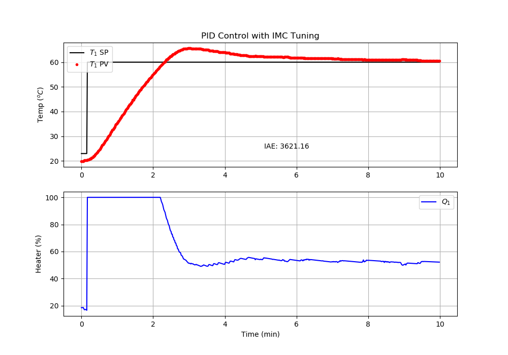
# Calculate Kc,tauI,tauD (IMC Aggressive)
# -----------------------------
tauc = max(0.1*taup,0.8*thetap)
Kc = (1/Kp)*(taup)/(thetap+tauc)
tauI = taup
tauD = 0
#------------------------
# PID Controller Function
#------------------------
# sp = setpoint
# pv = current temperature
# pv_last = prior temperature
# ierr = integral error
# dt = time increment between measurements
# outputs ---------------
# op = output of the PID controller
# P = proportional contribution
# I = integral contribution
# D = derivative contribution
def pid(sp,pv,pv_last,ierr,dt):
# Parameters in terms of PID coefficients
KP = Kc
KI = Kc/tauI
KD = Kc*tauD
# ubias for controller (initial heater)
op0 = 0
# upper and lower bounds on heater level
ophi = 100
oplo = 0
# calculate the error
error = sp-pv
# calculate the integral error
ierr = ierr + KI * error * dt
# calculate the measurement derivative
dpv = (pv - pv_last) / dt
# calculate the PID output
P = KP * error
I = ierr
D = -KD * dpv
op = op0 + P + I + D
# implement anti-reset windup
if op < oplo or op > ophi:
I = I - KI * error * dt
# clip output
op = max(oplo,min(ophi,op))
# return the controller output and PID terms
return [op,P,I,D]
n = 600 # Number of second time points (10 min)
tm = np.linspace(0,n-1,n) # Time values
lab = tclab.TCLab()
T1 = np.zeros(n)
Q1 = np.zeros(n)
# step setpoint from 23.0 to 60.0 degC
SP1 = np.ones(n)*23.0
SP1[10:] = 60.0
Q1_bias = 0.0
ierr = 0.0
iae = 0.0
for i in range(n):
# record measurement
T1[i] = lab.T1
iae += np.abs(SP1[i]-T1[i])
# --------------------------------------------------
# call PID controller function to change Q1[i]
# --------------------------------------------------
[Q1[i],P,ierr,D] = pid(SP1[i],T1[i],T1[max(0,i-1)],ierr,1.0)
lab.Q1(Q1[i])
if i%20==0:
print(' Heater, Temp, Setpoint')
print(f'{Q1[i]:7.2f},{T1[i]:7.2f},{SP1[i]:7.2f}')
# wait for 1 sec
time.sleep(1)
lab.close()
# Save data file
data = np.vstack((tm,Q1,T1,SP1)).T
np.savetxt('PI_control_IMC.csv',data,delimiter=',',\
header='Time,Q1,T1,SP1',comments='')
# Create Figure
plt.figure(figsize=(10,7))
ax = plt.subplot(2,1,1)
ax.grid()
plt.plot(tm/60.0,SP1,'k-',label=r'$T_1$ SP')
plt.plot(tm/60.0,T1,'r.',label=r'$T_1$ PV')
plt.text(4.1,26,'IAE: '+str(round(iae,2)))
plt.ylabel(r'Temp ($^oC$)')
plt.legend(loc=2)
ax = plt.subplot(2,1,2)
ax.grid()
plt.plot(tm/60.0,Q1,'b-',label=r'$Q_1$')
plt.ylabel(r'Heater (%)')
plt.xlabel('Time (min)')
plt.legend(loc=1)
plt.savefig('PI_Control_IMC.png')
plt.show()
import matplotlib.pyplot as plt
import tclab
import time
# process model
Kp = 0.9
taup = 175.0
thetap = 15.0
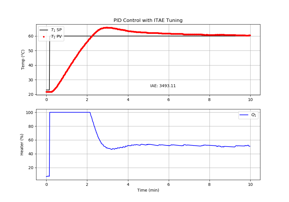
# -----------------------------
# Calculate Kc,tauI,tauD (ITAE)
# -----------------------------
Kc = (0.586/Kp)*(thetap/taup)**(-0.916)
tauI = taup/(1.03-0.165*(thetap/taup))
tauD = 0
#------------------------
# PID Controller Function
#------------------------
# sp = setpoint
# pv = current temperature
# pv_last = prior temperature
# ierr = integral error
# dt = time increment between measurements
# outputs ---------------
# op = output of the PID controller
# P = proportional contribution
# I = integral contribution
# D = derivative contribution
def pid(sp,pv,pv_last,ierr,dt):
# Parameters in terms of PID coefficients
KP = Kc
KI = Kc/tauI
KD = Kc*tauD
# ubias for controller (initial heater)
op0 = 0
# upper and lower bounds on heater level
ophi = 100
oplo = 0
# calculate the error
error = sp-pv
# calculate the integral error
ierr = ierr + KI * error * dt
# calculate the measurement derivative
dpv = (pv - pv_last) / dt
# calculate the PID output
P = KP * error
I = ierr
D = -KD * dpv
op = op0 + P + I + D
# implement anti-reset windup
if op < oplo or op > ophi:
I = I - KI * error * dt
# clip output
op = max(oplo,min(ophi,op))
# return the controller output and PID terms
return [op,P,I,D]
n = 600 # Number of second time points (10 min)
tm = np.linspace(0,n-1,n) # Time values
lab = tclab.TCLab()
T1 = np.zeros(n)
Q1 = np.zeros(n)
# step setpoint from 23.0 to 60.0 degC
SP1 = np.ones(n)*23.0
SP1[10:] = 60.0
Q1_bias = 0.0
ierr = 0.0
iae = 0.0
for i in range(n):
# record measurement
T1[i] = lab.T1
iae += np.abs(SP1[i]-T1[i])
# --------------------------------------------------
# call PID controller function to change Q1[i]
# --------------------------------------------------
[Q1[i],P,ierr,D] = pid(SP1[i],T1[i],T1[max(0,i-1)],ierr,1.0)
lab.Q1(Q1[i])
if i%20==0:
print(' Heater, Temp, Setpoint')
print(f'{Q1[i]:7.2f},{T1[i]:7.2f},{SP1[i]:7.2f}')
# wait for 1 sec
time.sleep(1)
lab.close()
# Save data file
data = np.vstack((tm,Q1,T1,SP1)).T
np.savetxt('PI_control_ITAE.csv',data,delimiter=',',\
header='Time,Q1,T1,SP1',comments='')
# Create Figure
plt.figure(figsize=(10,7))
ax = plt.subplot(2,1,1)
ax.grid()
plt.plot(tm/60.0,SP1,'k-',label=r'$T_1$ SP')
plt.plot(tm/60.0,T1,'r.',label=r'$T_1$ PV')
plt.text(4.1,26,'IAE: '+str(round(iae,2)))
plt.ylabel(r'Temp ($^oC$)')
plt.legend(loc=2)
ax = plt.subplot(2,1,2)
ax.grid()
plt.plot(tm/60.0,Q1,'b-',label=r'$Q_1$')
plt.ylabel(r'Heater (%)')
plt.xlabel('Time (min)')
plt.legend(loc=1)
plt.savefig('PI_Control_ITAE.png')
plt.show()
The simple_pid package gives a different solution for the PID validation with more overshoot, even with the same tuning parameters. There is a difference in how the PID equation is implemented. One of the advantages of the prior solutions is that the PID equation is easily inspected and modified. The advantage of using a standard PID package like simple_pid is that it reduces the implementation time and maintenance.
import time
import numpy as np
from simple_pid import PID
import matplotlib.pyplot as plt
# process model
Kp = 0.9
taup = 175.0
thetap = 15.0
c = ['IMC','ITAE']
for xi,ci in enumerate(c):
if ci=='IMC':
# -----------------------------
# Calculate Kc,tauI,tauD (IMC Aggressive)
# -----------------------------
tauc = max(0.1*taup,0.8*thetap)
Kc = (1/Kp)*(taup)/(thetap+tauc)
tauI = taup
tauD = 0
else:
# -----------------------------
# Calculate Kc,tauI,tauD (ITAE)
# -----------------------------
Kc = (0.586/Kp)*(thetap/taup)**(-0.916)
tauI = taup/(1.03-0.165*(thetap/taup))
tauD = 0
print('Controller Tuning: ' + ci)
print('Kc: ' + str(Kc))
print('tauI: ' + str(tauI))
print('tauD: ' + str(tauD))
lab = tclab.TCLab()
# Create PID controller
pid = PID(Kp=Kc,Ki=Kc/tauI,Kd=Kc*tauD,\
setpoint=23,sample_time=1.0,output_limits=(0,100))
n = 600
tm = np.linspace(0,n-1,n) # Time values
T1 = np.zeros(n)
Q1 = np.zeros(n)
# step setpoint from 23.0 to 60.0 degC
SP1 = np.ones(n)*23.0
SP1[10:] = 60.0
iae = 0.0
print('Time OP PV SP')
for i in range(n):
pid.setpoint = SP1[i]
T1[i] = lab.T1
iae += np.abs(SP1[i]-T1[i])
Q1[i] = pid(T1[i]) # PID control
lab.Q1(Q1[i])
print(i,round(Q1[i],2), T1[i], pid.setpoint)
time.sleep(pid.sample_time) # wait 1 sec
lab.close()
# Save data file
data = np.vstack((tm,Q1,T1,SP1)).T
np.savetxt('PID_control_'+ci+'.csv',data,delimiter=',',\
header='Time,Q1,T1,SP1',comments='')
# Create Figure
plt.figure(xi,figsize=(10,7))
ax = plt.subplot(2,1,1)
plt.title('PID Control with '+ci+' Tuning')
ax.grid()
plt.plot(tm/60.0,SP1,'k-',label=r'$T_1$ SP')
plt.plot(tm/60.0,T1,'r.',label=r'$T_1$ PV')
plt.text(5.1,25.0,'IAE: ' + str(round(iae,2)))
plt.ylabel(r'Temp ($^oC$)')
plt.legend(loc=2)
ax = plt.subplot(2,1,2)
ax.grid()
plt.plot(tm/60.0,Q1,'b-',label=r'$Q_1$')
plt.ylabel(r'Heater (%)')
plt.xlabel('Time (min)')
plt.legend(loc=1)
plt.savefig('PID_Control_'+ci+'.png')
print('Wait 10 min to cool down')
time.sleep(600)
plt.show()