Dynamics and Control

Objective: Determine the closed loop response of a PI controller to a step change in setpoint. Compare the analytical solution to the closed loop response to a setpoint change.

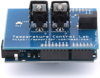
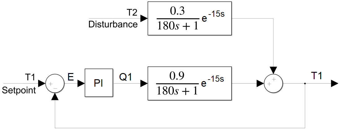
A TCLab block diagram shows the flow of information in a feedback control system that consists of a sensor, actuator, and controller. Block diagrams are different than a process diagram in that it is a diagram of the flow of information, not necessarily how the pieces of equipment are physically placed as reviewed in the TCLab Controller Assignment. The block diagram is a collection of signals and transfer functions that transform one signal into another. Transfer functions transform an input signal into an output signal. The PI controller (`K_c=2`, `\tau_I=180`) is a transfer function `G_c = K_c \frac{\tau_I s+1}{\tau_I s}` that tranforms an error signal (input) into a heater value (Q₁) (controller output). The process transfer function `(G_p = \frac{0.9}{180s+1} e^{-15s})` receives the heater value (Q₁) as an input and produces a change in temperature 1 (T_A1) process variable output. The disturbance transfer function `(G_d=\frac{0.3}{180s+1} e^{-15s})` has an input of temperature 2 (T₂) and produces a predicted change in temperature 1 (T_B1) process variable output. The two temperature outputs are added together as T₁ = T_A1 + T_B1. The loop is created with the sensor providing information to the controller as an error (E=T_SP-T₁) between the setpoint and measured value. The P-only controller changes the controller output Q₁ to change the temperature T₁ and the cycle starts again.

Block Diagram Algebra

The overall transfer function between the disturbance T₂ and T₁ is derived by algebraically combining the following expressions to eliminate all other signals besides the input and output of interest.

$$E(s) = T_{SP}(s)-T_1(s)$$

$$Q_1(s) = G_c(s) \, E(s) = G_c(s) \, (T_{SP}(s)-T_1(s))$$

$$T_{A1}(s) = G_p(s) \, Q_1(s) = G_c(s) \, G_p(s) \, (T_{SP}(s)-T_1(s))$$

$$T_{B1}(s) = G_d(s) \, T_2(s)$$

$$T_1(s) = T_{A1}(s)+T_{B1}(s) = G_c(s) \, G_p(s) \, (T_{SP}(s)-T_1(s)) + G_d \, T_2(s)$$

In this case, T_SP(s)=0 because it is assumed that there is no change in the setpoint as the disturbance transfer function is derived.

$$T_1(s) = - G_c(s) \, G_p(s) \, T_1(s) + G_d(s) \, T_2(s)$$

The transfer function is further simplified by collecting all T₁(s) terms to one side and T₂(s) terms to the other.

$$T_1(s) + G_c(s) \, G_p(s) , T_1(s) = G_d \, T_2(s)$$

This simplifies to the overall closed loop transfer function for disturbance changes.

$$\frac{T_1(s)}{T_2(s)} = \frac{G_d(s)}{1+G_c(s)\,G_p(s)} = \frac{\frac{0.3}{180s+1} e^{-15s}}{1+K_c \frac{\tau_I s+1}{\tau_I s} \frac{0.9}{180s+1} e^{-15s}}$$

Time-Delay to Polynomial Form

An inverse Laplace transform is not possible with this transfer function because of the exponential terms. To compute an analytical solution to a step input, a Taylor series approximation or Padé approximation of exp(-15s) with the first 2 or 3 terms are typically used to return to polynomial form.

Padé Approximation for exp

$$\exp(x) \approx \frac{1+\frac{1}{2}x+\frac{1}{9}x^2}{1-\frac{1}{2}x+\frac{1}{9}x^2}$$

Two terms are selected to approximate the dead-time. Additional terms improve the accuracy of the approximation but also increase the order of the polynomial.

$$\exp(-15s) \approx \frac{1-7.5 s}{1+7.5 s}$$

Taylor Series Approximation for exp

$$\exp(x) \approx \sum_{n=0}^{\infty}\frac{x^n}{n!} = 1+x+\frac{x^2}{2!}+\frac{x^3}{3!}+\dots$$

The exponential is first place in the denominator and two terms are selected to approximate the dead-time.

$$e^{-15s} = \frac{1}{e^{15s}} \approx \frac{1}{15s+1}$$

The Taylor series approximation is used for this example. The polynomial form of the transfer function is used for the analytical solution. The PI controller rejects the disturbance

Analytic Solution to PI Controller Response to +20^oC T₂ Disturbance

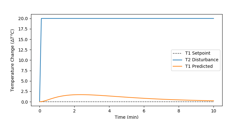
$$T(t) = \left(1.14 e^{0.0178t} - 7.97 e^{0.0600t} + 6.83 e^{0.067t}\right) e^{-0.072t} S(t-1)$$

Compute T₁ Analytic Solution to +20^oC Setpoint Change

Using the above as an example, calculate the closed loop transfer function for a PI controller between the other input (setpoint T_SP) and the output (T₁). Compute the analytical solution for T₁ and show predicted and measured values for a PI controller setpoint change from 23^oC to 43^oC. Use the PI Test Script to show the analytical and measured values for the closed loop control, modifying the line for the predicted temperature.

Solution

The overall transfer function between the disturbance T_SP and T₁ is derived by algebraically combining the same expressions to eliminate all other signals besides the input and output of interest.

$$E(s) = T_{SP}(s)-T_1(s)$$

$$Q_1(s) = G_c(s) \, E(s) = G_c(s) \, (T_{SP}(s)-T_1(s))$$

$$T_{A1}(s) = G_p(s) \, Q_1(s) = G_c(s) \, G_p(s) \, (T_{SP}(s)-T_1(s))$$

$$T_{B1}(s) = G_d(s) \, T_2(s)$$

$$T_1(s) = T_{A1}(s)+T_{B1}(s) = G_c(s) \, G_p(s) \, (T_{SP}(s)-T_1(s)) + G_d \, T_2(s)$$

In this case, T₂(s)=0 because it is assumed that there is no change in the disturbance as the setpoint transfer function is derived.

$$T_1(s) = G_c(s) \, G_p(s) \, (T_{SP}(s)-T_1(s))$$

The transfer function is further simplified by collecting all T₁(s) terms to one side and T_SP(s) terms to the other.

$$T_1(s) + G_c \, G_p(s) \, T_1(s) = G_c \, G_p(s) \, T_{SP}(s)$$

The closed loop transfer function is the ratio of the output to input.

$$\frac{T_1(s)}{T_{SP}(s)} = \frac{G_c \, G_p(s)}{1+G_c \, G_p(s)}$$

Analytic Solution to +20^oC Setpoint Change

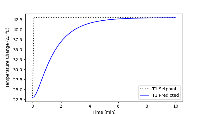
$$T(t) = \left( 20.0 + 6.14 e^{-0.054\,t} - 26.13 e^{-0.012\,t} \right) S(t-1)$$

import sympy as sym
from sympy.abc import s,t,x,y,z
import numpy as np
from sympy.integrals import inverse_laplace_transform
import matplotlib.pyplot as plt

# Define inputs
# Setpoint step (up) starts at 1 sec
TSP = 20/s*sym.exp(-s)

# Transfer functions
Kc = 2.0
tauI = 180.0
Gc = Kc * (tauI*s+1)/(tauI*s)
delay = 1/(15*s+1) # Taylor series approx
Gp = delay * 0.9/(180*s+1)

# Closed loop response
Gc = Gc*Gp/(1+Gc*Gp)

# Calculate response
T1 = Gc * TSP

# Inverse Laplace Transform
tsp = inverse_laplace_transform(TSP,s,t)
t1 = inverse_laplace_transform(T1,s,t)
print('Temperature Solution')
print(t1)

# generate data for plot
tm = np.linspace(0,600,100)
TSPplot = np.zeros(len(tm))
T1plot = np.zeros(len(tm))

# substitute numeric values
for i in range(len(tm)):
    TSPplot[i] = tsp.subs(t,tm[i]) + 23.0
    T1plot[i] = t1.subs(t,tm[i]) + 23.0

# plot results
plt.figure()
plt.plot(tm/60,TSPplot,'k:',label='T1 Setpoint')
plt.plot(tm/60,T1plot,'b-',label='T1 Predicted')
plt.legend()
plt.xlabel('Time (min)')
plt.ylabel(r'Temperature Change $(\Delta T \, ^oC)$')
plt.show()

[$[Get Code]]

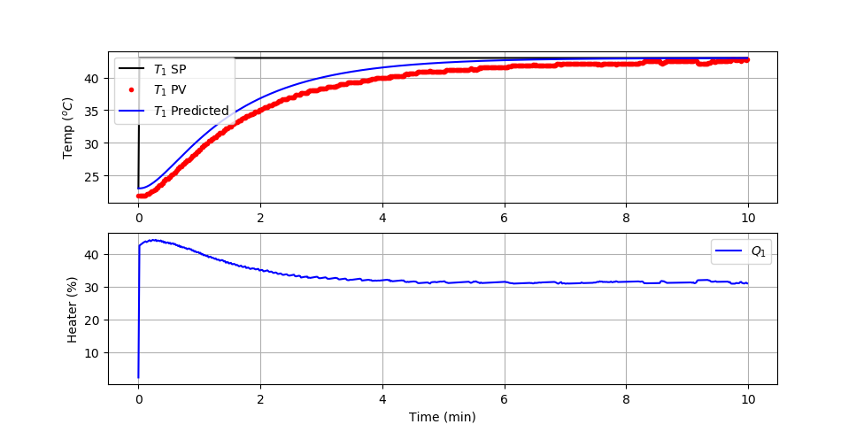
The PI Control test script is modified with the analytic solution.

T1Pred = 20 + 6.14*np.exp(-0.054*tm) - 26.13*np.exp(-0.012*tm) + 23.0

[$[Get Code]]

The plot shows a comparison of the predicted and measured temperature values. The ambient temperature is less than the 23^oC simulated value and can be adjusted to achieve a better match to the analytic solution. However, despite the offset, the measured dynamic response of the closed-loop response is similar to the analytic solution.