TCLab Higher Order Models
 |  |  |  |  |
|---|
Objective: Simulate a third-order transfer function, state space, and fifth-order time series model of TC2 temperature response to heater Q1.
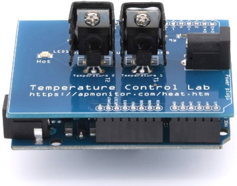
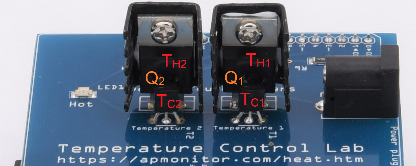
Higher-order models are better at predicting system dynamics for complex systems. This exercise is to create a third-order transfer function, state space, and a fifth-order time series model as linear representations of step response data. If heater 1 (Q1) controls temperature 2 (TC2), the generated heat first raises the heater 1 temperature (TH1). The heat is transferred by convection to heater 2 (TH2) and finally reaches temperature 2 sensor (TC2) by conduction. This heat transfer pathway suggests a third-order dynamic model, although a higher-order model may improve the fit even further.
Physics-Based Model
A physics-based model is developed in prior exercises as a second-order system. The second-order physics-based model consists of four differential equations from energy balances that include convection, conduction, and thermal radiation. There are three differential equations when considering the heat pathway from heater 1 (Q1) to temperature 2 sensor (TC2).
$$m\,c_p\frac{dT_{H1}}{dt} = U\,A\,\left(T_\infty-T_{H1}\right) + \epsilon\,\sigma\,A\,\left(T_\infty^4-T_{H1}^4\right) + Q_{C12} + Q_{R12} + \alpha_1 Q_1$$
$$m\,c_p\frac{dT_{H2}}{dt} = U\,A\,\left(T_\infty-T_{H2}\right) + \epsilon\,\sigma\,A\,\left(T_\infty^4-T_{H2}^4\right) - Q_{C12} - Q_{R12} + \alpha_2 Q_2$$
$$\tau \frac{dT_{C2}}{dt} = T_{H2} - T_{C2}$$
with the following heat transfer terms for simplifying the expressions.
$$Q_{C12} = U_s \, A_s \, \left(T_{H2}-T_{H1}\right)$$
$$Q_{R12} = \epsilon\,\sigma\,A_s\,\left(T_{H2}^4-T_{H1}^4\right)$$
$$\tau = \frac{m_s \, c_{p,s} \, \Delta x}{k\,A_c}$$
| Quantity | Value |
| Initial temperature (T0) | 293.15 K (20oC) |
| Ambient temperature (`T_\infty`) | 293.15 K (20oC) |
| Heater output (Q1) | 0-100 % |
| Heater factor (`\alpha_1`) | 0.0123 W/(% heater) |
| Heater output (Q2) | 0-100% |
| Heater factor (`\alpha_2`) | 0.0062 W/(% heater) |
| Heat capacity (Cp) | 500 J/kg-K |
| Surface Area Not Between Heaters (A) | 1.0x10⁻³ m2 (10 cm2) |
| Surface Area Between Heaters (As) | 2x10⁻⁴ m2 (2 cm2) |
| Mass (m) | 0.004 kg (4 gm) |
| Conduction Time Constant (tau) | 20.3 sec |
| Overall Heat Transfer Coefficient (U) | 4.7 W/m2-K |
| Overall Heat Transfer Coefficient Between Heaters (U_s) | 15.45 W/m2-K |
| Emissivity (`\epsilon`) | 0.9 |
| Stefan Boltzmann Constant (`\sigma`) | 5.67x10⁻⁸ W/m2-K4 |
import matplotlib.pyplot as plt
import pandas as pd
from gekko import GEKKO
import tclab
import time
# Import data
try:
# try to read local data file first
filename = 'data.csv'
data = pd.read_csv(filename)
except:
# heater steps
Q1d = np.zeros(601)
Q1d[10:200] = 80
Q1d[200:280] = 20
Q1d[280:400] = 70
Q1d[400:] = 50
Q2d = np.zeros(601)
try:
# Connect to Arduino
a = tclab.TCLab()
fid = open(filename,'w')
fid.write('Time,Q1,Q2,T1,T2\n')
fid.close()
# run step test (10 min)
for i in range(601):
# set heater values
a.Q1(Q1d[i])
a.Q2(Q2d[i])
print('Time: ' + str(i) + \
' Q1: ' + str(Q1d[i]) + \
' Q2: ' + str(Q2d[i]) + \
' T1: ' + str(a.T1) + \
' T2: ' + str(a.T2))
# wait 1 second
time.sleep(1)
fid = open(filename,'a')
fid.write(str(i)+','+str(Q1d[i])+','+str(Q2d[i])+',' \
+str(a.T1)+','+str(a.T2)+'\n')
# close connection to Arduino
a.close()
fid.close()
except:
filename = 'http://apmonitor.com/pdc/uploads/Main/tclab_data3.txt'
# read either local file or use link if no TCLab
data = pd.read_csv(filename)
# Fit Parameters of Energy Balance
m = GEKKO() # Create GEKKO Model
# Parameters to Estimate
U = m.FV(value=10,lb=1,ub=20)
Us = m.FV(value=20,lb=5,ub=40)
alpha1 = m.FV(value=0.01,lb=0.001,ub=0.03) # W / % heater
alpha2 = m.FV(value=0.005,lb=0.001,ub=0.02) # W / % heater
tau = m.FV(value=10.0,lb=5.0,ub=60.0)
# Measured inputs
Q1 = m.Param()
Q2 = m.Param()
Ta =20.0+273.15 # K
mass = 4.0/1000.0 # kg
Cp = 0.5*1000.0 # J/kg-K
A = 10.0/100.0**2 # Area not between heaters in m^2
As = 2.0/100.0**2 # Area between heaters in m^2
eps = 0.9 # Emissivity
sigma = 5.67e-8 # Stefan-Boltzmann
TH1 = m.SV()
TH2 = m.SV()
TC1 = m.CV()
TC2 = m.CV()
# Heater Temperatures in Kelvin
T1 = m.Intermediate(TH1+273.15)
T2 = m.Intermediate(TH2+273.15)
# Heat transfer between two heaters
Q_C12 = m.Intermediate(Us*As*(T2-T1)) # Convective
Q_R12 = m.Intermediate(eps*sigma*As*(T2**4-T1**4)) # Radiative
# Energy balances
m.Equation(TH1.dt() == (1.0/(mass*Cp))*(U*A*(Ta-T1) \
+ eps * sigma * A * (Ta**4 - T1**4) \
+ Q_C12 + Q_R12 \
+ alpha1*Q1))
m.Equation(TH2.dt() == (1.0/(mass*Cp))*(U*A*(Ta-T2) \
+ eps * sigma * A * (Ta**4 - T2**4) \
- Q_C12 - Q_R12 \
+ alpha2*Q2))
# Conduction to temperature sensors
m.Equation(tau*TC1.dt() == TH1-TC1)
m.Equation(tau*TC2.dt() == TH2-TC2)
# Options
# STATUS=1 allows solver to adjust parameter
U.STATUS = 1
Us.STATUS = 1
alpha1.STATUS = 1
alpha2.STATUS = 0
tau.STATUS = 1
Q1.value=data['Q1'].values
Q2.value=data['Q2'].values
TH1.value=data['T1'].values[0]
TH2.value=data['T2'].values[0]
TC1.value=data['T1'].values
TC1.FSTATUS = 1 # minimize fstatus * (meas-pred)^2
TC2.value=data['T2'].values
TC2.FSTATUS = 1 # minimize fstatus * (meas-pred)^2
m.time = data['Time'].values
m.options.IMODE = 5 # MHE
m.options.EV_TYPE = 2 # Objective type
m.options.NODES = 2 # Collocation nodes
m.options.SOLVER = 3 # IPOPT
m.solve(disp=False) # Solve physics-based model
# Parameter values
print('Estimated Parameters')
print('U : ' + str(U.value[0]))
print('Us : ' + str(Us.value[0]))
print('alpha1: ' + str(alpha1.value[0]))
print('alpha2: ' + str(alpha2.value[-1]))
print('tau: ' + str(tau.value[0]))
print('Constants')
print('Ta: ' + str(Ta))
print('m: ' + str(mass))
print('Cp: ' + str(Cp))
print('A: ' + str(A))
print('As: ' + str(As))
print('eps: ' + str(eps))
print('sigma: ' + str(sigma))
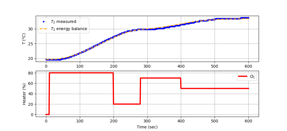
# Create plot
plt.figure(figsize=(10,7))
ax=plt.subplot(2,1,1)
ax.grid()
plt.plot(data['Time'],data['T2'],'b.',label=r'$T_2$ measured')
plt.plot(m.time,TC2.value,color='orange',linestyle='--',\
linewidth=2,label=r'$T_2$ energy balance')
plt.ylabel(r'T ($^oC$)')
plt.legend(loc=2)
ax=plt.subplot(2,1,2)
ax.grid()
plt.plot(data['Time'],data['Q1'],'r-',\
linewidth=3,label=r'$Q_1$')
plt.ylabel('Heater (%)')
plt.xlabel('Time (sec)')
plt.legend(loc='best')
plt.savefig('tclab_physics.png')
plt.show()
State Space Model
Below is a derivation of the state space and transfer function model of temperature 2 sensor response to heater 1 changes.
$$\begin{bmatrix}\dot T'_{H1}\\\dot T'_{H2}\\\dot T'_{C2}\end{bmatrix} = \begin{bmatrix}a_{1,1} & a_{1,2} & a_{1,3}\\a_{2,1} & a_{2,2} & a_{2,3}\\a_{3,1} & a_{3,2} & a_{3,3}\end{bmatrix} \begin{bmatrix}T'_{H1}\\T'_{H2}\\T'_{C2}\end{bmatrix} + \begin{bmatrix}b_{1,1}\\b_{2,1}\\b_{3,1}\end{bmatrix} \begin{bmatrix}Q'_1\end{bmatrix}$$
$$\begin{bmatrix}T'_{C2}\end{bmatrix} = \begin{bmatrix}0 & 0 & 1\end{bmatrix} \begin{bmatrix}T'_{H1}\\T'_{H2}\\T'_{C2}\end{bmatrix} + \begin{bmatrix}0\end{bmatrix} \begin{bmatrix}Q'_1\end{bmatrix}$$
In state space form:
$$\dot x = A x + B u$$
$$y = C x + D u$$
the individual elements are obtained by evaluating partial derivatives of the differential equations at steady state conditions.
$$a_{1,1} = \frac{\partial f_1}{\partial T_{H1}}\bigg|_{\bar Q,\bar T} = -\frac{U\,A + 4 \epsilon \sigma A T_0^3 + U_s \, A_s + 4 \epsilon \sigma A_s T_0^3}{m\,C_p} = -0.00698$$
$$a_{1,2} = \frac{\partial f_1}{\partial T_{H2}}\bigg|_{\bar Q,\bar T} = \frac{U_s \, A_s + 4 \epsilon \sigma A_s T_0^3}{m\,C_p} = 0.00206$$
$$a_{2,1} = \frac{\partial f_2}{\partial T_{H1}}\bigg|_{\bar Q,\bar T} = \frac{U_s \, A_s + 4 \epsilon \sigma A_s T_0^3}{m\,C_p} = 0.00206$$
$$a_{2,2} = \frac{\partial f_2}{\partial T_{H2}}\bigg|_{\bar Q,\bar T} = -\frac{U\,A + 4 \epsilon \sigma A T_0^3 + U_s \, A_s + 4 \epsilon \sigma A_s T_0^3}{m\,C_p} = -0.00698$$
$$a_{3,2} = \frac{\partial f_3}{\partial T_{H2}}\bigg|_{\bar Q,\bar T} = \frac{1}{\tau} = 0.0493$$
$$a_{3,3} = \frac{\partial f_3}{\partial T_{C2}}\bigg|_{\bar Q,\bar T} = -\frac{1}{\tau} = -0.0493$$
$$b_{1,1} = \frac{\partial f_1}{\partial Q_1}\bigg|_{\bar Q,\bar T} = \frac{\alpha_1}{m\,C_p} = 0.00616$$
The state space model has four matrices with `A` and `B` that are obtained from the partial derivatives of the right hand side of the differential equations.
$$A \in \mathbb{R}^{3 \, \mathrm{x} \, 3} = \begin{bmatrix}a_{1,1} & a_{1,2} & a_{1,3}\\a_{2,1} & a_{2,2} & a_{2,3}\\a_{3,1} & a_{3,2} & a_{3,3}\end{bmatrix} = \begin{bmatrix}-0.00698 & 0.00206 & 0\\0.00206 & -0.00698 & 0\\0 & 0.0493 & -0.0493\end{bmatrix}$$ $$B \in \mathbb{R}^{3 \, \mathrm{x} \, 1} = \begin{bmatrix}0.00616\\0\\0\end{bmatrix} $$ $$C \in \mathbb{R}^{1 \, \mathrm{x} \, 3} = \begin{bmatrix}0 & 0 & 1\end{bmatrix}$$ $$D \in \mathbb{R}^{1 \, \mathrm{x} \, 1} = \begin{bmatrix}0\end{bmatrix}$$
Use either Scipy.signal or Python Gekko to simulate the state space model with step input data.
Simulate State Space Model with Scipy.signal
t,y,x = signal.lsim(sys,u,t)
Simulate State Space Model with Python Gekko
x,y,u = ss.state_space(A,B,C,D=None)
ss.options.IMODE = 7
ss.solve(disp=False)
Transfer Function Model
An equivalent third-order transfer function model is obtained from the state space model.
$$G(s) = \frac{T_{C2}(s)}{Q_1(s)} = \frac{0.285}{456000s^3+28850s^2+334.1s+1}$$
Time Series Model
A fifth-order time series model is found by estimating `a_i` and `b_i` coefficients.
$$T_{C2,k+1} = \sum_{i=1}^{5} a_i T_{C2,k-i+1} + \sum_{i=1}^{5} b_i Q_{1,k-i+1}$$
Additional information on time series modeling is available with example code in Python Gekko.
Solution
Python Source Code
import matplotlib.pyplot as plt
import pandas as pd
from gekko import GEKKO
import tclab
import time
from scipy import signal
# Import data
try:
# try to read local data file first
filename = 'data.csv'
data = pd.read_csv(filename)
except:
filename = 'https://apmonitor.com/pdc/uploads/Main/tclab_data3.txt'
# read either local file or web file
data = pd.read_csv(filename)
U = 4.7052403301
Us = 15.45761703
alpha1 = 0.012321367852
alpha2 = 0.005
tau = 20.298826743
Ta = 293.15
mass = 0.004
Cp = 500.0
A = 0.001
As = 0.0002
eps = 0.9
sigma = 5.67e-08
Am = np.zeros((3,3))
Bm = np.zeros((3,1))
Cm = np.zeros((1,3))
Dm = np.zeros((1,1))
T0 = Ta
c1 = U*A
c2 = 4*eps*sigma*A*T0**3
c3 = Us*As
c4 = 4*eps*sigma*As*T0**3
c5 = mass*Cp
c6 = 1/tau
Am[0,0] = -(c1+c2+c3+c4)/c5
Am[0,1] = (c3+c4)/c5
Am[1,0] = (c3+c4)/c5
Am[1,1] = -(c1+c2+c3+c4)/c5
Am[2,1] = c6
Am[2,2] = -c6
Bm[0,0] = alpha1/c5
Cm[0,2] = 1
# state space simulation
ss = GEKKO(remote=False)
x,y,u = ss.state_space(Am,Bm,Cm,D=None)
u[0].value = data['Q1'].values
ss.time = data['Time'].values
ss.options.IMODE = 7
ss.solve(disp=False)
# state space simulation with scipy
sys = signal.StateSpace(Am,Bm,Cm,Dm)
tsys = data['Time'].values
Qsys = data['Q1'].values.T
tsys,ysys,xsys = signal.lsim(sys,Qsys,tsys)
# print linearized models
print('State Space Model')
print(sys)
print('Transfer Function Model')
tf=sys.to_tf()
print(tf)
# Time series model
ts = GEKKO(remote=False)
tt = data['Time'].values
tu = data['Q1'].values
ty = data['T2'].values
na = 5 # output coefficients
nb = 5 # input coefficients
print('Identify time series model')
# diaglevel = 1 option to see solver output
yp,p,K = ts.sysid(tt,tu,ty,na,nb,pred='model',objf=1000,diaglevel=0)
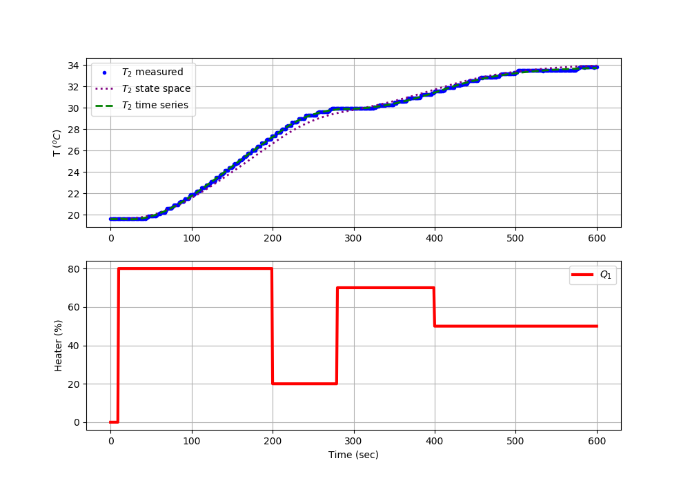
# Create plot
plt.figure(figsize=(10,7))
ax=plt.subplot(2,1,1)
ax.grid()
plt.plot(data['Time'],data['T2'],'b.',label=r'$T_2$ measured')
plt.plot(ss.time,np.array(y[0].value)+data['T2'][0],color='purple',linestyle=':',\
linewidth=2,label=r'$T_2$ state space')
plt.plot(tt,yp,'g--',\
linewidth=2,label=r'$T_2$ time series')
plt.ylabel(r'T ($^oC$)')
plt.legend(loc=2)
ax=plt.subplot(2,1,2)
ax.grid()
plt.plot(data['Time'],data['Q1'],'r-',\
linewidth=3,label=r'$Q_1$')
plt.ylabel('Heater (%)')
plt.xlabel('Time (sec)')
plt.legend(loc='best')
plt.savefig('tclab_higher_order.png')
plt.show()