Dynamics and Control

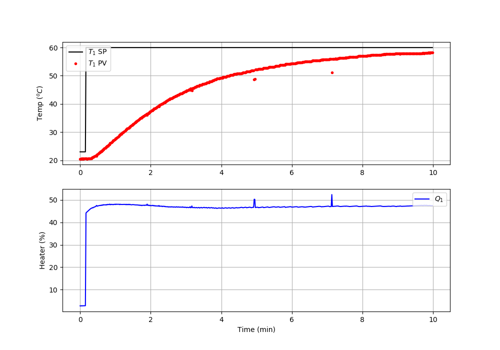
Objective: Implement a discrete PID controller without the derivative term (PI Control). Show the control performance with a setpoint change from 23^oC to 60^oC.

A proportional integral (PI) controller is a variation of the PID controller without the derivative term. The controller is an equation that adjusts the controller output, `u(t)`, for input into the system as the manipulated variable. It is a calculation of the difference between the setpoint SP and process variable PV. The adjustable parameters are the controller gain, `K_c`, and controller reset time or integral time constant, `\tau_I`. A large gain or small integral time constant produces a controller that reacts aggressively to a difference between the measured PV and target SP.

$$Q(t) = Q_{bias} + K_c \, \left( T_{SP}-T_{PV} \right) + \frac{K_c}{\tau_I}\int_0^t \left( T_{SP}-T_{PV} \right) dt $$

$$\quad = Q_{bias} + K_c \, e(t) + \frac{K_c}{\tau_I}\int_0^t e(t) dt$$

The `Q_{bias}` term is a constant that is typically set to the value of `Q(t)` when the controller is first switched from manual to automatic mode. The deviation variable for the heater is the change in value `Q'(t) = Q(t) - Q_{bias}`. For the TCLab, `Q_{bias}`=0 because the TCLab starts with the heater off. The `Q_{bias}` gives bumpless transfer if the error is zero when the controller is turned on. The error from the set point is the difference between the `T_{SP}` and `T_{PV}` and is defined as `e(t) = T_{SP} - T_{PV}`. The continuous integral is approximated in a discrete form as a summation of the error multiplied by the sample time.

$$\frac{K_c}{\tau_I}\int_0^t e(t) dt \approx \frac{K_c}{\tau_I} \sum_{i=1}^{n_t} e_i(t)\Delta t$$

See additional information on PI controllers. Use a basic tuning correlation with FOPDT parameters (`K_c` and `\tau_p`) determined from the TCLab graphical fitting or TCLab regression exercises.

$$K_c = \frac{1}{K_p} \quad \quad \tau_I = \tau_p$$

Fill in the values of `K_c`, `\tau_I`, and the PI equation in the code below. Add anti-reset windup to prevent the integral from accumulating when the heater is saturated at 0% or 100%.

Solution

import numpy as np
import matplotlib.pyplot as plt
import tclab
import time

# -----------------------------
# Input controller gain (Kc)
# Input controller time constant (tauI)
# -----------------------------
Kc = 1/0.9
tauI = 175.0

n = 600  # Number of second time points (10 min)
tm = np.linspace(0,n-1,n) # Time values
lab = tclab.TCLab()
T1 = np.zeros(n)
Q1 = np.zeros(n)
# step setpoint from 23.0 to 60.0 degC
SP1 = np.ones(n)*23.0
SP1[10:] = 60.0
Q1_bias = 0.0
ierr = 0.0
for i in range(n):
    # record measurement
    T1[i] = lab.T1

    # --------------------------------------------------
    # fill-in PI controller equation to change Q1[i]
    # --------------------------------------------------
    err = SP1[i]-T1[i]
    ierr += err
    Q1[i] = Q1_bias + Kc*err + Kc/tauI * ierr

    # --------------------------------------------------
    # implement new heater value with integral anti-reset windup
    if Q1[i]>=100:
        Q1[i]=100
        ierr -= err
    if Q1[i]<=0:
        Q1[i]=0
        ierr -= err
    # --------------------------------------------------

    lab.Q1(Q1[i])
    if i%20==0:
        print(' Heater,   Temp,  Setpoint')
    print(f'{Q1[i]:7.2f},{T1[i]:7.2f},{SP1[i]:7.2f}')
    # wait for 1 sec
    time.sleep(1)
lab.close()
# Save data file
data = np.vstack((tm,Q1,T1,SP1)).T
np.savetxt('PI_control.csv',data,delimiter=',',\
           header='Time,Q1,T1,SP1',comments='')

# Create Figure
plt.figure(figsize=(10,7))
ax = plt.subplot(2,1,1)
ax.grid()
plt.plot(tm/60.0,SP1,'k-',label=r'$T_1$ SP')
plt.plot(tm/60.0,T1,'r.',label=r'$T_1$ PV')
plt.ylabel(r'Temp ($^oC$)')
plt.legend(loc=2)
ax = plt.subplot(2,1,2)
ax.grid()
plt.plot(tm/60.0,Q1,'b-',label=r'$Q_1$')
plt.ylabel(r'Heater (%)')
plt.xlabel('Time (min)')
plt.legend(loc=1)
plt.savefig('PI_Control.png')
plt.show()

[$[Get Code]]