Modes
Main.Modes History
Hide minor edits - Show changes to markup
# GEKKO Python example for steady state optimization (imode=3)
# GEKKO Python example for steady state optimization (imode=3)
m.option.IMODE = 3
m.options.IMODE = 3
% MATLAB example for dynamic simulation (imode=7)
% APM MATLAB example for dynamic simulation (imode=7)
# Python example for model predictive control (imode=6)
# APM Python example for model predictive control (imode=6)
 # GEKKO Python example for steady state optimization (imode=3)
 from gekko import GEKKO
 m = GEKKO()
 m.option.IMODE = 3
APMonitor is designed to enable multiple modes of operation with one model. This model is defined in terms of differential and algebraic equations. The program handles all of the configuration and interfacing to the solvers. The simulation mode is changed with the nlc.imode option.
nlc.imode = {1-9}
APMonitor is designed to enable multiple modes of operation with one model. This model is defined in terms of differential and algebraic equations. The program handles all of the configuration and interfacing to the solvers. The simulation mode is changed with the APM.IMODE option.
IMODE = {1-9}
apm_option(server,app,'nlc.imode',7);
apm_option(server,app,'apm.imode',7);
apm_option(server,app,'nlc.imode',6)
apm_option(server,app,'apm.imode',6)
apm_option(server,app,'nlc.imode',6);
apm_option(server,app,'nlc.imode',6)
- Sequential dynamic estimation (SQE) - Newly Released on 22 Nov 2014
- Sequential dynamic optimization (SQO) - Newly Released on 22 Nov 2014
- Sequential dynamic estimation (SQE)
- Sequential dynamic optimization (SQO)
Modes of Operation
APMonitor is designed to enable multiple modes of operation with one model. This model is defined in terms of differential and algebraic equations. The program handles all of the configuration and interfacing to the solvers.
APMonitor is designed to enable multiple modes of operation with one model. This model is defined in terms of differential and algebraic equations. The program handles all of the configuration and interfacing to the solvers. The simulation mode is changed with the nlc.imode option.
 nlc.imode = {1-9}

 % MATLAB example for dynamic simulation (imode=7)
 apm_option(server,app,'nlc.imode',7);

 # Python example for model predictive control (imode=6)
 apm_option(server,app,'nlc.imode',6);
- Sequential dynamic estimation (SQE) - new 22 Nov 2014
- Sequential dynamic optimization (SQO) - new 22 Nov 2014
- Sequential dynamic estimation (SQE) - Newly Released on 22 Nov 2014
- Sequential dynamic optimization (SQO) - Newly Released on 22 Nov 2014
- Sequential dynamic estimation (SQE) - under development
- Sequential dynamic optimization (SQO) - under development
- Sequential dynamic estimation (SQE) - new 22 Nov 2014
- Sequential dynamic optimization (SQO) - new 22 Nov 2014
- Nonlinear control (CTL)
Modes 1-3 are steady state modes with all derivatives set equal to zero. Modes 4-6 are dynamic modes where the differential equations define how the variables change with time. Each mode has a steady state and dynamic option.
- Nonlinear control / dynamic optimization (CTL)
- Sequential dynamic simulation (SQS)
- Sequential dynamic estimation (SQE) - under development
- Sequential dynamic optimization (SQO) - under development
Modes 1-3 are steady state modes with all derivatives set equal to zero. Modes 4-6 are dynamic modes where the differential equations define how the variables change with time. Modes 7-9 are the same as 4-6 except the solution is performed with a sequential versus a simultaneous approach. Each mode for simulation, estimation, and optimization has a steady state and dynamic option.
Modes 2 and 5 are estimation modes. Mode 2 is for steady-state estimation and mode 5 is for dynamic estimation. Mode 2 is also known as the data reconciliation step in a real-time optimization solution. Mode 5 is also known as moving horizon estimation. Mode 5 is equivalent to the Kalman filter when the model is linear, the disturbance noise is white, and the probability distribution function is assumed Gaussian.
Modes 2 and 5 are estimation modes. Mode 2 is for steady-state estimation and mode 5 is for dynamic estimation. Mode 2 is also known as the data reconciliation step in a real-time optimization solution. Mode 5 is also known as moving horizon estimation. Mode 5 is equivalent to the Kalman filter when the model is linear, the disturbance noise is white, and the probability density function is assumed Gaussian.
- Nonlinear control (NLC)
- Nonlinear control (CTL)
- Moving horizon estimation (MHE)
- Moving horizon estimation (EST)
Modes 3 and 6 are optimization and control modes. Mode 3 performs steady-state optimization. Combined with mode 2, this constitutes a real-time optimization (RTO) solution. Mode 6 has a similar objective as mode 3 but is solved with a time-varying model. For linear models, this is often referred to as control. For nonlinear models, this is often referred to as nonlinear control (NLC) or nonlinear model predictive control (NMPC).
Modes 3 and 6 are optimization and control modes. Mode 3 performs steady-state optimization. Combined with mode 2, this constitutes a real-time optimization (RTO) solution. Mode 6 has a similar objective as mode 3 but is solved with a time-varying model. For linear models, this is often referred to as control. For nonlinear models, this is referred to as nonlinear control (NLC) or nonlinear model predictive control (NMPC).
- Simulation
Simulation
- Estimation
Estimation
- Optimization and Control
Optimization and Control
The core of all modes is the non-linear model. Each mode retrieves information from the non-linear model to give predictions or provides information to improve the model accuracy through parameter fitting.
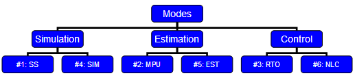
The core of all modes is the non-linear model. Each mode interacts with the nonlinear model to receive or provide information. There are 6 modes of operation for the APMonitor software.
- Steady-state simulation (SS)
- Model parameter update (MPU)
- Real-time optimization (RTO)
- Dynamic simulation (SIM)
- Moving horizon estimation (MHE)
- Nonlinear control (NLC)
Modes 1-3 are steady state modes with all derivatives set equal to zero. Modes 4-6 are dynamic modes where the differential equations define how the variables change with time. Each mode has a steady state and dynamic option.
- Simulation
Modes 1 and 4 are simulation-only modes. These simulation modes are for steady-state and dynamic investigation of the model. There is no optimization with the simulation modes. The model serves as a virtual process or simulator.
- Estimation
Modes 2 and 5 are estimation modes. Mode 2 is for steady-state estimation and mode 5 is for dynamic estimation. Mode 2 is also known as the data reconciliation step in a real-time optimization solution. Mode 5 is also known as moving horizon estimation. Mode 5 is equivalent to the Kalman filter when the model is linear, the disturbance noise is white, and the probability distribution function is assumed Gaussian.
- Optimization and Control
Modes 3 and 6 are optimization and control modes. Mode 3 performs steady-state optimization. Combined with mode 2, this constitutes a real-time optimization (RTO) solution. Mode 6 has a similar objective as mode 3 but is solved with a time-varying model. For linear models, this is often referred to as control. For nonlinear models, this is often referred to as nonlinear control (NLC) or nonlinear model predictive control (NMPC).
Non-linear Model Core
The core of all modes is the non-linear model. Each mode retrieves information from the non-linear model to give predictions or provides information to improve the model accuracy through parameter fitting.