Simulation
Dynamic Simulation
The DBS file parameter imode is used to control the simulation mode. This option is set to 4 (simultaneous simulation) or 7 (sequential simulation) for dynamic simulation.
 apm.imode = 4 (simultaneous dynamic simulation)
 apm.imode = 7 (sequential dynamic simulation)

 % MATLAB example
 apm_option(server,app,'apm.imode',7);

 # Python example
 apm_option(server,app,'apm.imode',4)
Like steady-state simulation, dynamic simulation requires a square problem with no degrees of freedom (neqn=nvar). Dynamic simulation has many useful purposes including
- Investigate step response characteristics of a nonlinear model
- Simulate process changes for design, trouble-shooting, or planning
- Perform what-if scenarios
- Simulate a virtual process
Dynamic simulation is the easiest dynamic mode to configure and run. The requirement for a square problem facilitates model convergence as the solver has only to achieve feasibility with the equality constraints.
Example Code (Python GEKKO) with IMODE 4 and 7
Three simulations show simultaneous simulation (IMODE=4), sequential simulation (IMODE=7), and simultaneous simulation in a Python loop (IMODE=4).
import numpy as np
import matplotlib.pyplot as plt
# Number of timesteps
nt = 11
tm = np.linspace(0, 1, nt)
# Initialize GEKKO
p1 = GEKKO()
p2 = GEKKO()
p3 = GEKKO()
# define model
for p in [p1,p2,p3]:
if p==p3:
p.time = [tm[0],tm[1]]
else:
p.time = tm
# Model parameters
p.g = p.Const(value=9.81, name='g')
p.l = p.Const(value=2., name='length')
p.m = p.Const(value=1.0, name='mass')
p.f = p.Const(value=0.5, name='friction coefficient')
# State Variables
p.theta = p.Var(value=0, name='angle')
p.dtheta_dt = p.Var(value=2.5, name='angular velocity')
# Equations
p.Equation(p.theta.dt() == p.dtheta_dt)
p.Equation(p.dtheta_dt.dt() == \
-p.g/p.l*p.sin(p.theta) - p.f/p.m*p.dtheta_dt)
p.options.NODES=5
# Solve simultaneously
p1.options.IMODE=4
p1.solve(disp=False)
p2.options.IMODE=7
p2.solve(disp=False)
p3.options.IMODE=4
th = np.ones_like(tm)
dth = np.ones_like(tm)
th[0] = 0
dth[0] = 2.5
import time
for i in range(1,nt):
p3.solve(disp=False)
# record values for plotting
th[i] = p3.theta.value[1]
dth[i] = p3.dtheta_dt.value[1]
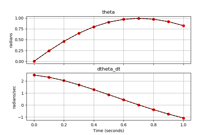
# Plot results
fig, axes = plt.subplots(2, 1, sharex=True, figsize=(8,7))
axes[0].plot(tm, p1.theta.value, 'o-',color='red')
axes[0].plot(tm, p2.theta.value, ':',color='green')
axes[0].plot(tm, th, '--',color='black')
axes[0].set_title("theta")
axes[0].set_ylabel('radians')
axes[0].grid()
axes[1].plot(tm, p1.dtheta_dt.value, 'o-',color='red')
axes[1].plot(tm, p2.dtheta_dt.value, ':',color='green')
axes[1].plot(tm, dth, '--',color='black')
axes[1].set_title("dtheta_dt")
axes[1].set_ylabel('radians/sec')
axes[1].grid()
axes[1].set_xlabel('Time (seconds)')
plt.show()