Solve 2nd Order Differential Equations
A differential equation relates some function with the derivatives of the function. Functions typically represent physical quantities and the derivatives represent a rate of change. The differential equation defines a relationship between the quantity and the derivative. Differential equations are very common in fields such as biology, engineering, economics, and physics.
Differential equations may be studied from several different perspectives. Only simple differential equations are solvable by explicit formulas while more complex systems are typically solved with numerical methods. Numerical methods have been developed to determine solutions with a given degree of accuracy.
The term with highest number of derivatives describes the order of the differential equation. A first-order differential equation only contains single derivatives. A second-order differential equation has at least one term with a double derivative. Higher order differential equations are also possible.
Second Order ODE Example
An example of a second-order differential equation with constant `K` and variable `y` with first derivative `y'` and second derivative `y''`:
$$y''+(0.9+0.7t)y' + K\,y = 0$$
and with initial conditions:
$$y(0)=2 \quad y'(0)=-1$$
Modified Form for Solution
To numerically solve a differential equation with higher-order (such as 2nd derivative) terms, it can be broken into multiple first-order differential equations by declaring a new variable `z` and equation `z=y'`. The modified problem is then:
$$z'+(0.9+0.7t)z + K\,y = 0$$
and with initial conditions:
$$y(0)=2 \quad z(0)=-1$$
A numerical solution to this equation can be computed with a variety of different solvers and programming environments. Solution files are available in MATLAB, Python, and Julia below or through a web-interface.
from gekko import GEKKO
import matplotlib.pyplot as plt
m = GEKKO(remote=False)
m.time = np.arange(0,2.01,0.05)
K = 30
y = m.Var(2.0)
z = m.Var(-1.0)
t = m.Var(0.0)
m.Equation(t.dt()==1)
m.Equation(y.dt()==z)
m.Equation(z.dt()+(0.9+0.7*t)*z+K*y==0)
m.options.IMODE = 4; m.options.NODES = 3
m.solve(disp=False)
plt.plot(m.time,y.value,'r-',label='y')
plt.plot(m.time,z.value,'b--',label='z')
plt.legend()
plt.xlabel('Time')
plt.show()
Each of these example problems can be modified for solutions to other second-order differential equations as well.

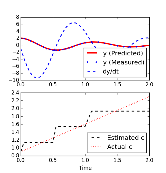
Another scenario is when the damping coefficient c = (0.9 + 0.7 t) is not known but must be estimated from data. The value of c is allowed to change every 0.5 seconds. The true and estimated values of c are shown on the plot below. Predicted and actual values of y are in agreement even though the estimate is not continuous but only changes at discrete time points.